

Data Modeling in Power BI: Joins, Relationships, and Schemas
Introduction
Data modeling is the process of organizing your data into tables, defining relationships between them, and enhancing the data with calculated fields, measures, and hierarchies. This process ensures accurate analysis and sets you up to create clear, impactful Power BI reports.
Types of SQL Joins
Joins are one of the most important features that SQL offers. Joins allow us to make use of the relationships we have set up between our tables.
In this article, we’ll break down the core SQL join types:
1. INNER JOIN
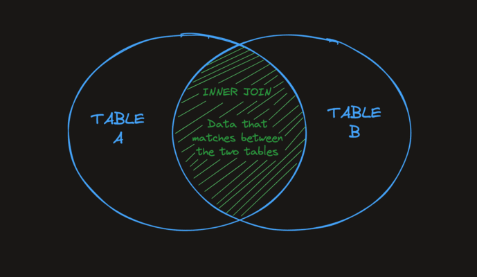
The SQL INNER JOIN statement joins two tables based on a common column and selects rows that have matching values in these columns.

Example:
SELECT *
FROM employees
INNER JOIN departments
ON employees.department_id = departments.id;
In this query:
employees.department_id refers to the department_id column from the employees table.
departments.id refers to the id column from the departments table.
The ON clause ensures that rows are matched based on these columns, creating a relationship between the two tables.
The query above returns all the fields from both tables. The INNER keyword only affects the number of rows returned, not the number of columns. The INNER JOIN filters rows based on matching department_id and id, while the SELECT * ensures all columns from both tables are included.
2. LEFT JOIN
The SQL LEFT JOIN combines two tables based on a common column. It then selects records having matching values in these columns and the remaining rows from the left table.

Example:
-- left join Customers and Orders tables based on their shared customer_id columns
-- Customers is the left table
-- Orders is the right table

SELECT Customers.customer_id, Customers.first_name, Orders.item
FROM Customers
LEFT JOIN Orders
ON Customers.customer_id = Orders.customer_id;
Here, the SQL command combines data from the Customers and Orders tables.
The query selects the customer_id and first_name from Customers and the amount from Orders.
Hence, the result includes rows where customer_id from Customers matches customer from Orders.
3. RIGHT JOIN
The SQL RIGHT JOIN statement joins two tables based on a common column. It selects records that have matching values in these columns and the remaining rows from the right table.

Case Example
-- join Customers and Orders tables
-- based on customer_id of Customers and customer of Orders
-- Customers is the left table
-- Orders is the right table

SELECT Customers.customer_id, Customers.first_name, Orders.amount
FROM Customers
RIGHT JOIN Orders
ON Customers.customer_id = Orders.customer;
Here, the SQL command selects the customer_id and first_name columns (from the Customers table) and the amount column (from the Orders table).
And, the result set will contain those rows where there is a match between customer_id (of the Customers table) and customer (of the Orders table), along with all the remaining rows from the Orders table.
4. FULL OUTER JOIN
The SQL FULL OUTER JOIN statement joins two tables based on a common column. It selects records that have matching values in these columns and the remaining rows from both of the tables.

Use Case Example
SELECT Customers.customer_id, Customers.first_name, Orders.amount
FROM Customers
FULL OUTER JOIN Orders
ON Customers.customer_id = Orders.customer;
Here, the SQL command selects the customer_id and first_name columns (from the Customers table) and the amount column (from the Orders table).
The result set will contain all rows of both the tables, regardless of whether there is a match between customer_id (of the Customers table) and customer (of the Orders table).
5. ANTI JOIN
- The SQL
LEFT ANTI JOINreturns rows in the left table that have no matching rows in the right table.
How it works:
Achieved withLEFT JOIN+WHERE [key in right table] IS NULL. - The SQL
RIGHT ANTI JOINreturns rows in the right table that have no matching rows in the left table.
How it works:
Achieved withRIGHT JOIN+WHERE [key in left table] IS NULL.
Case Example
SELECT *
FROM tableA
LEFT JOIN tableB ON tableA.key = tableB.key
WHERE tableB.key IS NULL;
This query will return all rows from tableA that do not have a corresponding row in tableB
CARDINALITY
In Power BI, the term “cardinality” describes the type of relationship between two tables according to how many related rows each table has. It specifies the relationships between rows in one table and rows in another.
-
One-to-Many (1 : *): In this relationship, one record in the first table connects to many records in the second table.
Example:
Each customer can have multiple orders, but each order belongs to only one customer.
In the model view, this appears as 1 –> *
The “1” side is usually a dimension table (like Customers).
The “many” side is a fact table (like Orders). -
Many-to-One (* : 1): This is the reverse direction of a one-to-many relationship. It happens when the filter starts from the many side and moves to the one side.
Example:
If you select a particular order in a visual (from the Orders table), Power BI can trace it back to the correct Customer in the Customers table.
Multiple orders (many) point to one customer (one), that is a many-to-one relationship. -
One-to-One (1 : 1): Each record in one table matches exactly one record in another table.
Example:
Assume, you have a Customer table and a Customer Profile table. Each customer ID appears only once in both tables.
Useful when you split a large table into smaller parts for better performance. -
Many-to-Many (* : *): Both tables can have repeating values in their key columns
Example:
Imagine you are a student and you want to join club, each student can join multiple clubs and each club can have multiple students.
Power BI manages this scenario using a bridge table, which maps each student to each club.
Active Vs. Inactive Relationships
Active
An active relationship in Power BI is the primary, default connection between two tables. Power BI automatically uses active relationships for filtering and calculations unless you specify otherwise.
You can only have one active relationship between two tables at a time, even if there are multiple potential ways they could be related.
Example:
Consider a Sales table and a Dates table. You might have a relationship based on the OrderDate field. If this is the main date you want to use for your analysis, it will be marked as the active relationship.
Inactive
An inactive relationship is a secondary connection between two tables that Power BI does not automatically use for filtering or calculations. These relationships are useful when you need multiple ways to connect tables, but only one connection should be used by default.
Inactive relationships can be activated manually in specific measures or calculations using DAX (Data Analysis Expressions).
Example:
In addition to OrderDate, your Sales table might also have a ShipDate field that relates to the Dates table. You can create an inactive relationship between ShipDate and Dates, which you can activate selectively when needed.
CROSS FILTER
Cross filtering in Power BI determines how filters are applied across related tables in a relationship. It defines the direction in which the filter context flows between tables.
There are two types of cross filter direction:
-
Single Direction:
Filters flow from one table to another, for example: from Customer to Orders.
This is the default and most efficient setup. -
Both Direction/Bidirectional:
Filters flow both ways between tables.
Used when both tables should influence each other, for example: Region and Sales.
How Cardinality and Cross Filtering work together
Cardinality defines how tables are connected, while cross filtering defines how filters move through those connections. Together, they ensure that your visuals respond correctly to user actions.
Example:
Cardinality: One-to-Many between Customers and Orders.
Cross Filter Direction: Single from Customers to Orders.
Result: Selecting a customer filters their orders but not the other way around.
Difference between Relationships and Joins
Relationships:
- Are displayed as flexible noodles between logical tables
- Require you to select matching fields between two logical tables
- Do not require you to select join types
- Make all row and column data from related tables potentially available in the data source
- Maintain each table’s level of detail in the data source and during analysis
- Create independent domains at multiple levels of detail. Tables aren’t merged together in the data source.
- During analysis, create the appropriate joins automatically, based on the fields in use.
- Do not duplicate aggregate values (when Performance Options are set to Many-to-Many)
- Keep unmatched measure values (when Performance Options are set to Some Records Match)
Joins:
- Are displayed with Venn diagram icons between physical tables
- Require you to select join types and join clauses
- Joined physical tables are merged into a single logical table with a fixed combination of data
- May drop unmatched measure values
- May duplicate aggregate values when fields are at different levels of detail
- Support scenarios that require a single table of data, such as extract filters and aggregation
Fact Vs. Dimension Tables
| Characteristic | Fact Table | Dimension Table |
|---|---|---|
| Basic Definition | It contains data (often transactional) that you want to analyze | It accompanies the fact table and stores information that describe records in the fact table |
| Purpose | It contains measures and is used for analysis and decision making | It contains information about a business and its process |
| Type of Data | Numeric and textual format | Textual format |
| Primary/Foreign Key | A primary key for each dimension which is acts as a foreign key in the dimension table | A foreign key associated with the primary key of the fact table |
| Hierarchy | No hierarchy | Contains a hierarchy |
| Attributes | Less attributes | More Attributes |
| Records | More Records | Less Records |
| Table Growth | Grows vertically | Grows horizontally |
| Data Model | Fewer fact tables in the data model | More dimension tables in a data model |
| Update Frequency | Records added very frequently | Records not added frequently |
Star Schema
A star schema is a way to organize data in a database, especially in data warehouses, to make it easier and faster to analyze. At the center, there’s a main table called the fact table, which holds measurable data. Around it are dimension tables.

Snowflake Schema
A snowflake schema splits dimension tables into smaller sub-dimensions to keep data more organized and detailed; just like snowflakes in a large lake.

Flat Table
A flat table in Power BI is a single, wide table containing all data, including measures and descriptive attributes, without relationships, similar to a spreadsheet.
| OrderID | Date | Product | Category | Customer | Region | Qty | Unit Price |
|---|---|---|---|---|---|---|---|
| 1001 | 01/01/26 | Laptop | Electronics | Alice | North | 1 | 1000 |
| 1002 | 01/02/26 | Desk | Furniture | Bob | South | 2 | 150 |
| 1003 | 01/02/26 | Laptop | Electronics | Charlie | North | 1 | 1000 |
Role-playing Dimensions
Role-playing dimensions in Power BI occur when a single dimension table (e.g. Date) connects to a fact table multiple times, representing different roles (e.g. Order Date, Ship Date). Power BI allows only one active relationship between tables; subsequent roles are inactive.
Common Modeling Issues
- Building Models from CSV exports.
- Missing Unique Keys.
- Using Multiple date tables.
- Overlapping attributes across tables.
- Lack of normalisation.
- Ignoring virtual relationships.
- Keeping unnecessary columns.
Conclusion
I hope you found this blog helpful in understanding the significance of data modeling and the basic principles crucial to building an effective data model. By understanding these fundamental concepts, such as star schemas, cardinality, cross-filter direction, and active and inactive relationships, you should be well on your way to becoming a more proficient Power BI developer.



 Avatar: The Last Airbender dizisinin 2. sezonuyla ekranlara döneceği tarih belli oldu. Netflix, merakla beklenen yeni sezonun yayın tarihini yeni bir tanıtım videosu paylaşarak duyurdu.

 Samsung, araç yolculuklarında görülen “taşıt tutması” sorununu azaltmayı hedefleyen yeni bir Android uygulaması tanıttı.

 Fujitsu, tamamen Japonya’da geliştirilecek 1.4 nm yapay zeka çipi için düğmeye bastı. Çipin üretimi için Rapidus’a başvurulurken maliyetin 58 milyar yen seviyesinde olması bekleniyor.

 Superman ile başlatılan yeni DC Sinematik Evreni’nin ikinci filmi olan Supergirl’den yeni bir fragman yayınlandı. Milly Alcock’un başrolünü üstlendiği film, 26 Haziran’da vizyona girecek.

 Bu yaz vizyona girecek Masters of the Universe filminden yeni fragman geldi. He-Man, Amazon tarafından hazırlanan bu büyük bütçeli filmle yıllar sonra sinemalara dönecek.

 Airbnb, tek noktadan seyahat platformu olma yolunda attığı bir diğer adım olarak yeni özel araç karşılama hizmetini tanıttı. Bu özellik dünya genelinde 125 şehirde kullanıma sunulacak.