The Problem

In my previous post, I shared how I used an AI agent framework during a train ride to build a Proof of Concept (POC) for a project called the Dog Finder App. The response was great, but the experiment raised a technical question: How do you build a POC quickly without creating a messy monolith that you’ll have to rewrite later?

When building a data-intensive application, engineers usually face a harsh trade-off. You can either build it fast to prove the concept (and inherit massive technical debt), or you can build it “right” (and spend weeks provisioning infrastructure and writing boilerplate).

By leveraging serverless services on Google Cloud Platform (GCP), we can break that trade-off.

This is the first in a three-part series where I will show you how to architect, automate, and deploy a complete, decoupled data application. We will look at how combining serverless tools with strict Data Engineering practices allows you to spin up a solution that is both incredibly fast to build and ready for production traffic.

The Architecture: Decoupling by Default

In traditional POCs, it is common to see a tightly coupled monolith: a single backend service receiving HTTP requests, saving images to a local disk, writing state to a database, and running heavy analytical queries. If one component bottlenecks, the entire application crashes.

For the Dog Finder app—a system designed to ingest real-time sightings of lost dogs and route them for geographical analysis—we needed a system that scales instantly under load but costs absolutely nothing when there is no traffic.

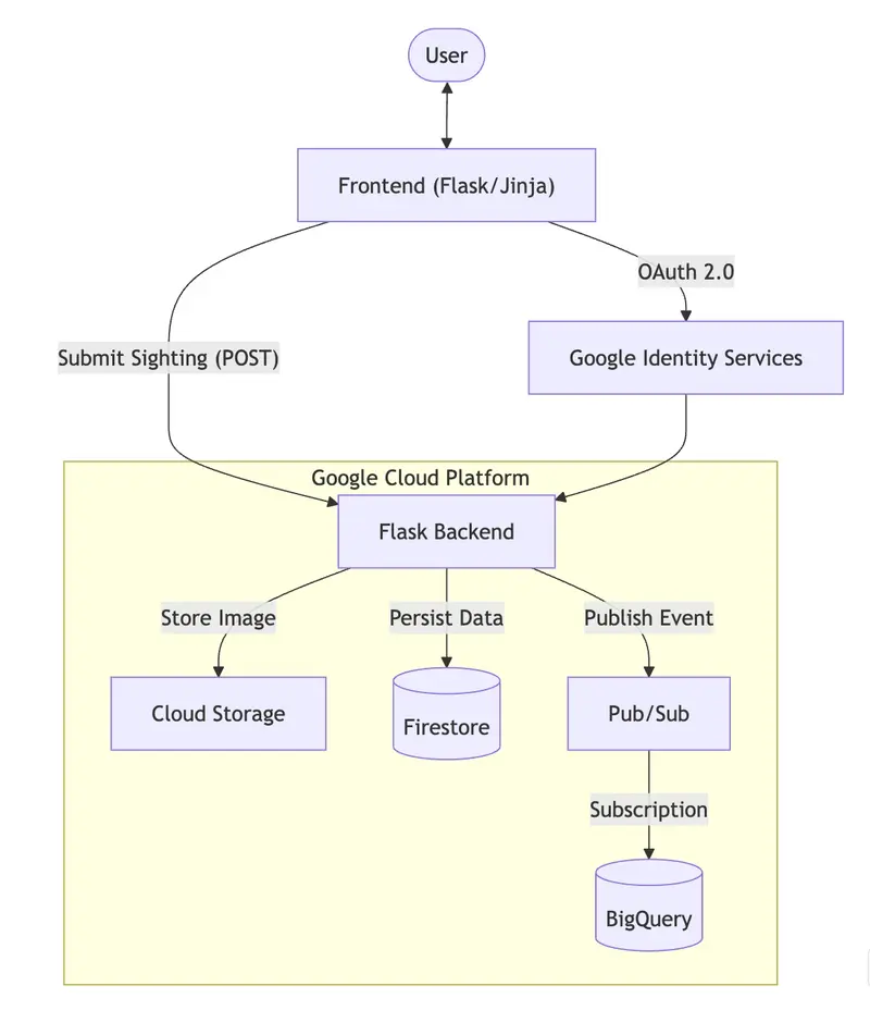
To achieve this, we default to a decoupled architecture. We split the ingestion, state, and analytics across specialized, managed serverless components:

• Google Cloud Run (Compute): Hosts our stateless Flask web application and API. It handles incoming user traffic, scales up automatically on demand, and drops to zero when idle.
• Google Cloud Storage (Blob Storage): Handles the heavy payloads. User-uploaded images of dogs go straight here, keeping our databases lean and performant.

• Firestore (Operational Database): Our OLTP layer. This NoSQL database stores the real-time state of the application, allowing the frontend to read and display current sightings with millisecond latency.

• Cloud Pub/Sub (Ingestion Buffer): The shock absorber of our system. When a sighting occurs, the backend publishes an event here and immediately responds to the user, completely decoupling the web app from the analytics pipeline.

• BigQuery (Data Warehouse): Our OLAP layer. The final destination where all structured sightings land for historical storage, regional partitioning, and complex analytical querying.

The Compute Layer: Scaling to Zero with Cloud Run

At the core of the Dog Finder app is a Python Flask backend. In a traditional setup, you would provision a Virtual Machine (Compute Engine) to run this application. You’d pay for that VM 24/7, even at 3:00 AM when no one is reporting lost dogs.

Instead, we containerized the application using a standard Dockerfile and deployed it to Google Cloud Run.

Cloud Run is a fully managed compute platform that automatically scales stateless containers. As an architect, enforcing statelessness is critical here. The Flask app does not store any session data or images on its local filesystem. Its only job is to act as a highly efficient traffic cop:

• Receive the HTTP POST request (the sighting payload and image).
• Validate the data payload.
• Offload the heavy lifting to our specialized data services.
• Return a success response to the user.

If there is a massive spike in lost dog reports, Cloud Run spins up multiple container instances instantly. When traffic drops, it scales down to zero. We only pay for the exact number of milliseconds the CPU spends processing a request.

The Data Split: OLTP vs. OLAP in a Serverless World

This is where many rapid POCs turn into unmaintainable monoliths. A common mistake is throwing all your data—images, real-time app state, and analytical history—into a single relational database like PostgreSQL. As the application grows, database locks increase, queries slow down, and storage costs skyrocket.

To prevent this, we split the data path into three specialized lanes:

1. Cloud Storage (The Payload)

Databases are expensive places to store binary files. When a user uploads a photo of a dog, our Cloud Run app sends that file directly to a Google Cloud Storage bucket. The app then grabs the resulting image_url and uses that string for the rest of the data pipeline. This keeps our databases incredibly lean and fast.

2. Firestore (Operational / OLTP)

Users expect a snappy UI. When they open the app, they want to see the latest dog sightings immediately. We use Firestore (a NoSQL document database) as our operational layer. After saving the image, Cloud Run writes the sighting record to Firestore. This provides low-latency reads and writes, ensuring the web frontend feels instantaneous without running complex SQL joins.

3. BigQuery (Analytical / OLAP)

While Firestore is great for the UI, it is not designed for heavy aggregations (e.g., “How many Golden Retrievers were lost in the northern region last month compared to last year?”).

For this, we route the data to BigQuery. We explicitly partitioned the BigQuery table by sighting_date. This is a crucial Data Engineering standard: when analysts query the table for recent trends, BigQuery only scans the relevant partitions, drastically reducing query costs and execution time.

The Payoff: Visualizing the Data (Looker Studio)

An architecture is only as good as the insights it delivers. The real payoff of this decoupled, partitioned setup became obvious when I wanted to add a visualization layer.

Because we cleanly separated our operational state (Firestore) from our analytical history (BigQuery), I was able to connect Looker Studio directly to the BigQuery table in minutes. I didn’t have to worry about complex API integrations or degrading the performance of the live web app.

I created a real-time dashboard that plots the sightings by region. As new records flow through the serverless pipeline, the dashboard updates automatically, providing a live heat map of lost dog hotspots. This transforms the POC from a simple “data entry” app into a complete, end-to-end data product.

Conclusion & What’s Next

In this first part, we laid out the “boxes” of our architecture. By leveraging Cloud Run, Cloud Storage, Firestore, and BigQuery, we designed a system that scales instantly, costs nothing when idle, and handles both operational and analytical workloads perfectly.

But having the right boxes is only half the battle. How do we connect them reliably?

In Part 2, we will dive into the lines connecting the boxes. I will show you how to use Pub/Sub to fully decouple ingestion, how to set up a direct serverless subscription from Pub/Sub to BigQuery (no code required), and how to enforce strict Data Contracts so your beautiful data warehouse doesn’t turn into a data swamp.

What is Quantum Computing?

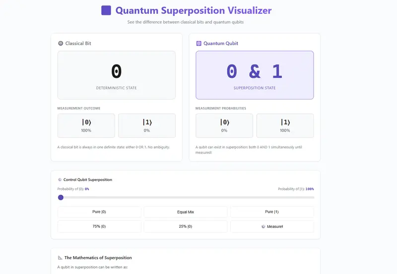
At its core, Quantum Computing is a fundamentally different way of processing information. While classical computers (the one you’re using right now) use bits—which are always either a 0 or a 1—quantum computers use qubits.

Qubits exploit the strange laws of quantum mechanics, specifically:

• Superposition: A qubit can exist as both 0 and 1 simultaneously until it is measured.
• Entanglement: Two qubits can become linked such that the state of one instantly influences the state of the other, no matter the distance.

These properties allow quantum computers to explore a vast “probability space” all at once, potentially solving problems in chemistry, cryptography, and optimization that would take classical supercomputers thousands of years to calculate.

The Building Blocks: Circuits and Gates

To perform a calculation on a quantum computer, we build a Quantum Circuit.

• Quantum Wires: The horizontal lines in a diagram represent the timeline of a single qubit.
• Quantum Gates: These are the “operations” we perform on qubits to change their state. Think of them like the logical AND/OR/NOT gates in a classical computer, but with a quantum twist:
  • Hadamard (H): Puts a qubit into a perfect 50/50 superposition of 0 and 1.
  • Pauli-X (X): The quantum version of a NOT gate; it flips a bit from 0 to 1.
  • CNOT (Controlled-NOT): The builder of entanglement! It flips a target qubit only if the control qubit is 1.
• Measurement: This is the final step where the quantum “magic” ends and we collapse the superposition into a classical 0 or 1 that we can read.

Enter: Quantum Studio

Learning these concepts is notoriously difficult. The math is complex, and the assembly code (OpenQASM) can be cryptic for beginners.

I built Quantum Studio to be the bridge between human intent and quantum logic.

If you wnat to use NVIDIA you can get key here https://build.nvidia.com/explore/discover?ncid=ref-inpa-550095

🤖 Why I Created It

I wanted to learn quantum computing in a truly visual and intuitive way. I realized that the best way to understand an entanglement circuit is to see it being built gate-by-gate.

Quantum Studio helps you master quantum theory through:

1. AI-Powered Intent: You don’t need to know the code. Just type “Make a Bell State and measure both qubits” and the AI handles the translation.
2. Live Visualizations: As soon as the logic is generated, it’s rendered on a clean, modern canvas. No more abstract math; you see the wires and gates.
3. Real-Time Animation: Use the Animate feature to watch the evolution of the circuit step-by-step. It helps you build a mental map of how information flows through the system.
4. Open Source Education: By turning Natural Language (NLP) into standard OpenQASM 2.0, Quantum Studio teaches you the underlying code automatically as you experiment.

Quantum computing will redefine the next several years of technology. Quantum Studio is my contribution to making that future accessible to everyone—not just PhDs.

🎓 Learning Quantum Computing Interactively

To make quantum concepts truly accessible, I’ve created 10 interactive visualizers that let you learn by doing rather than by memorizing. Each visualizer focuses on a specific concept, transforming abstract mathematics into intuitive, hands-on experiences.

Why Interactive Learning Works

Research consistently shows that interactive visualization improves learning outcomes by 30-60% compared to passive reading. When learning quantum computing:

• You can’t truly understand superposition until you manipulate probability amplitudes yourself
• You can’t grasp the Bloch sphere until you rotate it and apply gates in 3D
• You can’t comprehend measurement collapse until you watch it happen in real-time
• You can’t master quantum algorithms until you step through them gate-by-gate

Traditional textbooks present quantum mechanics as pure theory. Interactive visualizers let you play first, then formalize the concepts with mathematics.

🎯 The Complete Visualizer Suite

All visualizers are free, open-source, and work directly in your browser—no installation required. Here’s what you can explore:

Foundational Concepts (Perfect for Beginners)

1. Superposition Visualizer

https://vishalmysore.github.io/QuantumStudio/superposition_visualizer.html

• See the fundamental difference between classical bits and quantum qubits
• Adjust probability amplitudes with interactive sliders
• Watch wave functions evolve in real-time
• Simulate measurements and see quantum randomness
• Start here if you’re completely new to quantum computing

1. Interactive Bloch Sphere

https://vishalmysore.github.io/QuantumStudio/bloch_sphere_interactive.html

• Visualize single-qubit states in beautiful 3D
• Drag to rotate the sphere from any angle
• Apply quantum gates (H, X, Y, Z) and watch states transform
• Control theta and phi angles manually
• Quick presets for common states (|0⟩, |1⟩, |+⟩, |−⟩)
• Essential for understanding quantum state geometry

1. Measurement Collapse Visualizer 📏

https://vishalmysore.github.io/QuantumStudio/measurement_collapse_visualizer.html

• Watch superposition collapse into definite states
• 3-stage timeline: Before → Measurement → After
• Run 100 measurements to see statistical distributions
• Histogram showing probability convergence
• Demonstrates the mysterious measurement problem

1. Gate Transformer 🎛️

https://vishalmysore.github.io/QuantumStudio/gate_transformer_visualizer.html

• Apply quantum gates one by one
• See transformation flow: Input → Gate → Output
• Compare probabilities before and after
• View gate matrix representations
• Build gate sequences with history tracking
• Learn how gates transform quantum states

Multi-Qubit Systems (Intermediate Level)

1. Multi-Qubit Explorer 🔗

https://vishalmysore.github.io/QuantumStudio/multi_qubit_explorer.html

• Switch between 1, 2, and 3 qubits
• Experience exponential state space growth (2, 4, 8 states)
• Visualize all basis states with amplitude bars
• Entanglement indicators show quantum correlations
• Quick access to Bell and GHZ states
• Understand why quantum computers scale exponentially

1. Bell State Visualizer 🔗

https://vishalmysore.github.io/QuantumStudio/bell_state_visualizer.html

• Create quantum entanglement between two qubits
• 4-step process showing entanglement creation
• Visual qubit spheres with connection animation
• Measurement correlation matrix
• See Einstein’s “spooky action at a distance”
• Your first hands-on entanglement experience

Quantum Algorithms (Advanced Implementations)

7.Deutsch’s Algorithm ⚡

https://vishalmysore.github.io/QuantumStudio/deutsch_algorithm_visualizer.html

• The first algorithm to prove quantum advantage
• Toggle between Constant and Balanced functions
• Oracle truth table display
• 4-step walkthrough with phase visualization
• Determine function type in one query instead of two
• See quantum computing’s computational advantage

1. Grover’s Search Algorithm 🔍

https://vishalmysore.github.io/QuantumStudio/grovers_algorithm_visualizer.html

• Search unsorted database in √N time instead of N time
• 5-step animation: Init → Superposition → Oracle → Diffusion → Measure
• Amplitude and probability bars for all states
• Phase visualization showing oracle marking
• Word search demo (find “paneer” at index 2)
• Master amplitude amplification techniques

1. Quantum Teleportation Visualizer 📡
   https://vishalmysore.github.io/QuantumStudio/teleportation_visualizer.html

• Transfer quantum states using entanglement
• Alice and Bob party representation
• 6-step protocol showing the complete process
• Entanglement channel animation
• Classical communication (2 bits) visualization
• Advanced quantum protocol in action

1. GHZ State Visualizer 🐱

https://vishalmysore.github.io/QuantumStudio/ghz_state_visualizer.html

- Create "Schrödinger's Cat" states with 3, 4, or 5 qubits
- Maximum multi-qubit entanglement
- Dynamic step generation based on qubit count
- Qubit chain visualization
- Amplitude distribution grid
- Formula: (|000...⟩ + |111...⟩)/√2
- **Explore multi-party entanglement**

📚 Recommended Learning Path

For Complete Beginners:

1. Superposition Visualizer → Understand qubits vs bits
2. Bloch Sphere → Visualize quantum states
3. Gate Transformer → Learn gate operations  
4. Measurement Collapse → See quantum randomness
5. Multi-Qubit Explorer → Understand scaling
6. Bell State → Experience entanglement
7. Deutsch's Algorithm → See quantum advantage
8. Grover's Algorithm → Amplitude amplification
9. Teleportation → Advanced protocols
10. GHZ State → Multi-party entanglement

Original Japanese article: AWSのレイクハウス（Apache Iceberg）をSnowflakeと連携する2つのパターンを整理する

Introduction

I’m Aki, an AWS Community Builder (@jitepengin).

In recent years, it has become increasingly common to build lakehouse architectures centered around Apache Iceberg.

Before the rise of lakehouse architecture, it was common to design systems where data was consolidated into a specific platform, such as:

• an architecture centered around Amazon Redshift on AWS
• an architecture centered around internal tables in Snowflake

However, with the advent of Apache Iceberg, this assumption is rapidly changing.

Now that data on Amazon S3 can be directly accessed from multiple engines, what matters is no longer simply product selection.
Instead, the architecture design itself has become the central focus: where the data resides, who owns the write responsibility, and who holds governance authority.

In this article, focusing on the coexistence of AWS and Snowflake, I will organize the following:

• two patterns based on S3 × Iceberg
• connectivity with Power BI Service
• future prospects including AI utilization

Why AWS × Snowflake Coexistence Is Necessary

The greatest value of Apache Iceberg lies in its ability to separate data from the query engine.

For example, while keeping the physical data stored in S3, the same data can be accessed from multiple tools such as Athena, AWS Glue / Spark, Redshift, and Snowflake.

In other words, while consolidating the physical data into a single location, it has become possible to choose the most suitable analytics platform depending on the use case.

As a result, the architectural discussion has shifted from “which product should we use?” to “where should data sovereignty reside, and where should analytical ownership be placed?”

The benefits of using Snowflake here include:

• user-friendly UI/UX
• powerful SQL analytics capabilities
• integration with Cortex AI

In particular, I believe that an architecture where AWS serves as the data sovereignty layer while Snowflake is utilized as the analytics layer is highly compatible.

Two Patterns for Snowflake × S3 Integration

Here, I will organize the two commonly used patterns when integrating Snowflake with S3.

Pattern 1: Glue Catalog Integration

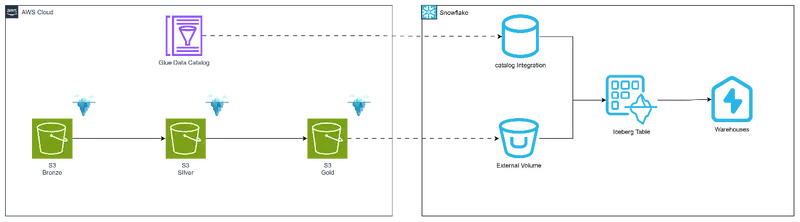
In this pattern, Iceberg tables stored on S3 are referenced from Snowflake through AWS Glue Data Catalog.

The advantages of this architecture are:

• relatively simple configuration
• S3 becomes the Single Source of Truth
• because Snowflake cannot write, AWS retains sovereignty over data management
  (this can also be considered a disadvantage)
• since user access is consolidated into Snowflake, access control can be centralized there

In other words, Snowflake focuses solely on the role of data analytics (query engine), while AWS retains authority over data management.

Setup Procedure

Step 1: Create an External Volume (S3 Access Configuration)

Run the following on the Snowflake side:

CREATE EXTERNAL VOLUME IF NOT EXISTS sample_iceberg_volume
  STORAGE_LOCATIONS = (
    (
      NAME = 'my-s3-location'
      STORAGE_PROVIDER = 'S3'
      STORAGE_BASE_URL = catalog S3 path
      STORAGE_AWS_ROLE_ARN = role ARN to use
      STORAGE_AWS_EXTERNAL_ID = 'my_external_id'
    )
  );

Step 2: Create Glue Catalog Integration

Run the following on the Snowflake side:

CREATE OR REPLACE CATALOG INTEGRATION glue_catalog_int -- arbitrary name
  CATALOG_SOURCE = GLUE
  CATALOG_NAMESPACE = Glue catalog namespace
  TABLE_FORMAT = ICEBERG
  GLUE_AWS_ROLE_ARN = role ARN to use
  GLUE_CATALOG_ID = Glue catalog ID to use
  GLUE_REGION = 'ap-northeast-1'
  ENABLED = TRUE;

Step 3: Retrieve Required Information for AWS Trust Policy

DESC EXTERNAL VOLUME sample_iceberg_volume;

→ Note down STORAGE_AWS_IAM_USER_ARN and STORAGE_AWS_EXTERNAL_ID

DESC CATALOG INTEGRATION glue_catalog_int;

→ Note down GLUE_AWS_IAM_USER_ARN and GLUE_AWS_EXTERNAL_ID

Since the two External IDs above will have different values, be sure to add both to the AWS IAM role Trust Policy.

Please configure the Trust Policy for the role used on the AWS side.

{
    "Version": "2012-10-17",
    "Statement": [
        {
            "Effect": "Allow",
            "Principal": {
                "AWS": STORAGE_AWS_IAM_USER_ARN
            },
            "Action": "sts:AssumeRole",
            "Condition": {
                "StringEquals": {
                    "sts:ExternalId": STORAGE_AWS_EXTERNAL_ID
                }
            }
        },
        {
            "Effect": "Allow",
            "Principal": {
                "AWS": GLUE_AWS_IAM_USER_ARN
            },
            "Action": "sts:AssumeRole",
            "Condition": {
                "StringEquals": {
                    "sts:ExternalId": GLUE_AWS_EXTERNAL_ID
                }
            }
        }
    ]
}

Step 4: Create Database

Run the following on the Snowflake side:

CREATE DATABASE IF NOT EXISTS icebergdb;

Step 5: Create Table

Run the following on the Snowflake side:

CREATE OR REPLACE ICEBERG TABLE icebergdb.public.yellow_tripdata -- arbitrary name
  EXTERNAL_VOLUME = 'sample_iceberg_volume'
  CATALOG = 'glue_catalog_int'
  CATALOG_TABLE_NAME = 'yellow_tripdata'
  AUTO_REFRESH = TRUE;

Step 6: Verify Data

Run the following on the Snowflake side:

SELECT * FROM icebergdb.public.yellow_tripdata LIMIT 5;

We were able to read the data from S3!

Pattern 2: Catalog-Linked Database (Iceberg)

This pattern integrates Glue Catalog using the REST Catalog approach and manages Iceberg tables directly from the Snowflake side.

The advantages of this architecture are:

• read and write operations from Snowflake are possible
• the physical data remains stored in S3
• Snowflake users can perform SQL-based updates and analytics
• easier integration with Power BI and Cortex AI

In other words, the biggest feature is that analysis and updates can be performed from Snowflake while keeping the physical data in S3.

However, governance must be considered from both the AWS side and the Snowflake side.

Setup Procedure

Step 1: Create an External Volume (S3 Access Configuration)

CREATE EXTERNAL VOLUME IF NOT EXISTS sample_iceberg_volume
  STORAGE_LOCATIONS = (
    (
      NAME = 'my-s3-location'
      STORAGE_PROVIDER = 'S3'
      STORAGE_BASE_URL = catalog S3 path
      STORAGE_AWS_ROLE_ARN = role ARN to use
      STORAGE_AWS_EXTERNAL_ID = 'my_external_id'
    )
  );

Step 2: Create Glue Iceberg REST Catalog Integration

CREATE OR REPLACE CATALOG INTEGRATION glue_rest_catalog_int
  CATALOG_SOURCE = ICEBERG_REST
  TABLE_FORMAT = ICEBERG
  CATALOG_NAMESPACE = Glue catalog namespace
  REST_CONFIG = (
    CATALOG_URI = Glue catalog URI
    CATALOG_API_TYPE = AWS_GLUE
    CATALOG_NAME = AWS account ID
  )
  REST_AUTHENTICATION = (
    TYPE = SIGV4
    SIGV4_IAM_ROLE = role ARN to use
    SIGV4_SIGNING_REGION = 'ap-northeast-1'
  )
  ENABLED = TRUE;

Step 3: Retrieve Required Information for AWS Trust Policy

DESC EXTERNAL VOLUME sample_iceberg_volume;

→ Note down STORAGE_AWS_IAM_USER_ARN and STORAGE_AWS_EXTERNAL_ID

DESC CATALOG INTEGRATION glue_rest_catalog_int;

→ Note down GLUE_AWS_IAM_USER_ARN and GLUE_AWS_EXTERNAL_ID

Since the two External IDs above will have different values, be sure to add both to the AWS IAM role Trust Policy.

Please configure the Trust Policy for the role used on the AWS side.

{
    "Version": "2012-10-17",
    "Statement": [
        {
            "Effect": "Allow",
            "Principal": {
                "AWS": STORAGE_AWS_IAM_USER_ARN
            },
            "Action": "sts:AssumeRole",
            "Condition": {
                "StringEquals": {
                    "sts:ExternalId": STORAGE_AWS_EXTERNAL_ID
                }
            }
        },
        {
            "Effect": "Allow",
            "Principal": {
                "AWS": GLUE_AWS_IAM_USER_ARN
            },
            "Action": "sts:AssumeRole",
            "Condition": {
                "StringEquals": {
                    "sts:ExternalId": GLUE_AWS_EXTERNAL_ID
                }
            }
        }
    ]
}

Step 4: Create Catalog Linked Database (Read/Write Enabled)

CREATE DATABASE my_iceberg_linked_db
  LINKED_CATALOG = (
    CATALOG = 'glue_rest_catalog_int',
    ALLOWED_WRITE_OPERATIONS = ALL
  )
  EXTERNAL_VOLUME = 'sample_iceberg_volume';

Step 5: Tables Are Automatically Discovered (Synced Every 30 Seconds)

SELECT * FROM my_iceberg_linked_db."icebergdb"."yellow_tripdata" LIMIT 5;

We were able to read the data from S3!

Step 6: Write Test

INSERT INTO my_iceberg_linked_db."icebergdb"."yellow_tripdata"
  (vendorid, tpep_pickup_datetime, tpep_dropoff_datetime, passenger_count,
   trip_distance, ratecodeid, store_and_fwd_flag, pulocationid, dolocationid,
   payment_type, fare_amount, extra, mta_tax, tip_amount, tolls_amount,
   improvement_surcharge, total_amount, congestion_surcharge, airport_fee)
VALUES
  (1, '2025-01-01 13:00:00', '2025-01-01 13:30:00', 2,
   3.5, 1, 'N', 100, 200,
   1, 15.0, 2.5, 0.5, 3.0, 0,
   1.0, 22.0, 2.5, 0);

Step 7: Verify Write

SELECT * FROM my_iceberg_linked_db."icebergdb"."yellow_tripdata"
WHERE tpep_pickup_datetime = '2025-01-01 13:00:00';

We were able to write data into S3!

Athena side

Before write

After write

Which Pattern Should You Choose?

For practical use, the following way of organizing it is easy to understand.

Integration with Power BI Service

Traditionally, when referencing an S3-based lakehouse from Power BI Service, many architectures used Redshift as an intermediary.

In such cases, securely connecting directly from Power BI Service often required provisioning an EC2 instance and configuring an on-premises data gateway.

This introduces additional operational costs such as EC2 management.

Now, how about Snowflake?

Power BI provides a native connector for Snowflake, allowing direct authentication and connection from Power BI Service.

This eliminates the need for relay servers or on-premises gateways that are often required in Redshift-based architectures.

In other words, it becomes possible to exclude costly operational components such as on-premises gateways.

In addition, since the semantically organized Gold layer on the Snowflake side can be directly connected to Power BI, this also improves usability for BI users.

Thinking in Terms of Medallion Architecture

Personally, I consider the following architecture to be highly practical for real-world use.

• Bronze: S3 + Iceberg
• Silver: S3 + Iceberg (with Snowflake integration as needed)
• Gold: S3 + Iceberg → Snowflake integration

By especially aligning the Gold layer with Snowflake, it becomes easier to provide a semantic layer that is easy for BI users and business departments to consume.

Depending on the use case, the Silver layer can also be utilized for more detailed analysis.

In other words, this enables a separation of responsibilities between data management and data analytics.

Thinking in Terms of Separation of Ownership

This is the most important point in this article.

What matters is not the product itself, but how ownership is separated.

By clearly defining this separation, it becomes easier to organize the scope of responsibilities across data engineering, BI, and AI utilization, which also provides benefits from an organizational management perspective.

The Change Brought by Snowflake Cortex AI

AI utilization will become even more important going forward.

As with other data platforms, AI adoption is progressing rapidly in Snowflake as well.

By leveraging Snowflake Cortex AI, it becomes possible to query Iceberg tables on S3 using natural language.

In other words, the data platform is evolving from “a platform for writing SQL” into “a platform for conversation.”

AI utilization is expected to continue evolving in many aspects.

One key point will be preparing data that is easier for AI to use—in other words, AI-ready data.

Conclusion

In this article, I organized two patterns for integrating an AWS lakehouse (Apache Iceberg) with Snowflake.

In recent data utilization scenarios, it is increasingly common not only to rely solely on AWS, but also to integrate with platforms such as Databricks and Snowflake as introduced here.

As mentioned earlier, what matters is not the product itself, but how ownership is separated.

Depending on which service takes responsibility for data, governance, and analytics, both the architecture and configuration will change.

In any case, what is truly important is not the product itself, but the perspective of how to design a data platform that users will continue to use over time.

Going forward, it will become even more important to design architectures not only from the perspective of where data is stored, but also from the viewpoint of who owns responsibility for each layer and how that responsibility connects to user value.

I hope this article will be helpful for those considering a combination of AWS and Snowflake.

51万行源码泄露：全面解构 Claude Code 如何成为 AI 编程天花板

原文链接：https://warpnav.com/claude-code-source-map

2026年3月31日，安全研究者 Chaofan Shou 发现了一个“史诗级”的构建疏漏。 Anthropic 发布到 npm 的 Claude Code (v2.1.88) 包体积从 17MB 暴涨到了 31MB。多出来的部分，是一个重达 60MB 的 source map 文件（cli.js.map）。这意味着什么？这意味着 Anthropic 忘了剥离调试文件，导致 Claude Code 完整的 TypeScript 源码——整整 51.2 万行，1903（或 1906）个源文件——完全暴露在了公网上。

有意思的是，2025 年 2 月 Claude Code 刚上 npm 时就犯过一模一样的错误。虽然这不涉及模型权重，对普通用户没有安全风险，但这却给全世界的 AI 开发者提供了一份价值连城的“内部技术架构图”。

当你翻开这包含 API 设计、遥测系统、加密工具、IPC 协议的 51 万行代码，带着“为什么它就是比别人好用”的疑问去阅读时，你会得出一个震撼的结论：这不是一个 AI 编程助手，这是一个以 LLM 为内核的操作系统。

一、系统架构：这不是 CLI 工具，而是运行平台

大多数人对 AI 编程工具的理解停留在表面：用户输入 → 调用 LLM API → 返回代码显示。如果你照着这个思路去复刻，出来的体验和 Claude Code 会有天壤之别。

想象一下你雇了一个远程程序员来操作你的电脑：

• Cursor 的做法： 让他坐在你旁边，敲命令前你看一眼，点个“允许”。简单粗暴，但费神。
• GitHub Copilot Agent 的做法： 给他一台新虚拟机随便折腾，搞完提交代码。安全，但脱离了你本地的真实环境。
• Claude Code 的做法： 让他直接用你的电脑，但配了一套极其精密的安检系统。他想用 rm -rf 都要经过 9 层审查。

从源码目录 src/ 的顶层结构来看，它的复杂程度令人咋舌：入口层、常量与提示词、工具定义、运行时服务、命令系统、UI 组件、协调器、记忆系统、插件、Hook 系统、任务系统一应俱全。

它拥有四个独立入口（CLI、初始化流程、MCP 模式、SDK），同一个 Agent 运行时可以服务四种交互界面，这是典型的平台化设计标志。它的命令系统不仅内建了 /mcp, /memory, /tasks 等十几个系统级命令，还统一加载动态技能，本身就是一个庞大的生态入口。

二、提示词工程：一台精密的“动态组装机器”

大多数人以为 System Prompt（系统提示词）是一大段固定的文本，启动时塞进去就完事了。但 Claude Code 的提示词是由 getSystemPrompt() 函数动态拼装出来的，更像是一个编译器的输出。

它的拼装逻辑分为两个截然不同的部分：

1. 静态部分（系统的“宪法”）

这部分无论什么会话都不会改变，包括身份定位、系统规范、做任务的哲学、风险动作规范、工具使用规范和语气风格等。

2. 动态部分（系统的“当期政策”）

这部分每次对话都不同，会动态注入：会话引导、记忆片段、环境信息、你的 CLAUDE.md 项目配置、MCP 插件说明，甚至是 Token 预算和输出风格。

核心秘密在于“缓存边界”与 Token 经济学：
源码中有一个名为 SYSTEM_PROMPT_DYNAMIC_BOUNDARY 的标记。

• 边界之上的内容是静态的，API 可以完美缓存它们，这既节省了大量 Token 费用，又极大提升了响应速度。
• 边界之下的内容是动态的，确保每次对话都能感知当前环境。
  当你的产品每天要处理海量请求时，这种把提示词当做预算来管理的“上下文经济学”直接决定了产品的生死。

三、铁血行为约束：如何管教 AI 不乱来？

你一定遇到过这种崩溃场景：让 AI 改个小 Bug，它顺手把半个文件重构了，还加了五个你不需要的错误处理。Claude Code 怎么解决？靠的是把规矩写成“铁律”。

1. 细致入微的“任务哲学”

在 getSimpleDoingTasksSection() 模块中，Anthropic 给模型立下了严苛的规矩：

• 不要加用户没要求的功能。
• 不要过度抽象，不要瞎重构。
• 不要乱加注释和文档字符串。
• 不要给时间估计。
• 方法失败时先诊断原因再换策略，删除确认没用的东西，绝不搞兼容性垃圾。
• 结果要如实汇报，不能假装自己测试过了。

2. 工具使用的“语法规则”

工具规范被写得极其死板：

• 读文件必须用 FileRead，不许用 cat/head/tail。
• 改文件必须用 FileEdit，不许用 sed/awk（正则写错容易崩）。
• 没有依赖关系的工具调用必须并行处理。

3. 每个工具都有独立的“使用手册”

系统有 42 个工具，但它们是按需延迟加载的，只有需要时才通过 ToolSearchTool 注入，以节省 Token。每个工具目录下都有专门写给 AI 看的 prompt.ts。
例如 BashTool 的手册明确规定了 Git 安全协议：

• 绝对不要擅自 git push --force 或 reset --hard。
• 强制：总是创建新的 commit 而不是 amending。

此外，系统采用 Fail-closed（默认封闭）设计。在工具工厂函数中，isConcurrencySafe 和 isReadOnly 默认全是 false。这意味着如果开发者忘了声明安全属性，系统宁可误杀也会将其视为“有风险、会写入”的工具，绝不漏掉一个风险。同时，FileEditTool 强制要求必须先使用 FileReadTool，没读过文件就去盲改会直接报错拦截。

(注：源码中甚至还有 USER_TYPE === 'ant' 的分支，专门给 Anthropic 内部员工提供更激进的输出策略和实验功能。)

四、多 Agent 分发与 14 步执行流水线

当任务复杂时，Claude Code 不会单打独斗，而是生成一个子 Agent 蜂群（Swarm）。源码确认了至少六个内建 Agent，包括通用、探索、计划、验证等。

1. 角色隔离原则

• Explore Agent（探索） & Plan Agent（计划）： 被设计成纯只读模式。它们不能创建、修改或移动文件，连执行 Bash 也只限于 ls 或 git status。规划和实现彻底分开，防止 AI 在探索阶段不小心改坏代码。
• 防偷懒与自我意识注入： 主 Agent 派发任务时，被严格限制不允许写“基于你的发现去修 bug”这种模糊指令，必须给出具体的行号和路径。而子 Agent 启动时会被注入：“你是一个工人，不是经理。不要交流，直接干活，严禁再生成子代”，切断了无限递归的可能。
• Coordinator 模式（协调器）： 主 Agent 变身项目经理，分配 3 个 worker 并行搜索代码库，2 个 worker 串行修改不同文件避免冲突，并行成为它的超能力。为了最大化子 Agent 缓存命中率，所有 Fork 出来的任务都会统一使用 'Fork started — processing in background' 作为文本前缀，巧妙利用字节级前缀匹配白嫖缓存。

2. 整个系统最值钱的设计：Verification Agent

人类自己 Review 代码都会因为疲惫而敷衍，LLM 更是如此。Verification Agent（验证专家）的指令堪称全场最狠：

• 核心方向是 “try to break it”（想办法搞坏它）。
• 严厉打击“只看代码不跑检查”的逃避行为，或者被“UI 看起来还行”迷惑的偷懒倾向。
• 强制要求跑 Build、跑测试套件、跑 Linter。前端要跑浏览器自动化，后端要用 curl 实测响应，甚至要做 adversarial probes（对抗性探测）去寻找边界破绽。
• 它和写代码的 Agent 利益隔离，没有“自我感觉良好”的偏见，只负责冷酷地给出 PASS、FAIL 或 PARTIAL 判决。

3. 工具调用的 14 步治理流水线

工具不是说调就调的。当 AI 决定使用工具时，要经过一条漫长的治理流水线：
解析输入 → 校验 Schema → 跑内部 validateInput → 跑投机分类器（Speculative classifier）预判风险 → 执行 PreToolUse Hook（可改写输入或拦截） → 进入正式权限决策 → 二次修正输入 → 真正执行 tool.call() → 记录遥测日志 → 执行 PostToolUse Hook → 处理结构化输出（成功或失败都有对应 Hook 收尾）。
这就是把“默认一切都会出问题”刻在了骨子里。

五、 永不超限的三层压缩机制

长对话一定会导致 Token 爆炸。Claude Code 如何让对话“永不超限”还能“记住你”？

1. 仿生学的记忆与 KAIROS “做梦”模式

• 它使用另一个小模型（Claude Sonnet）来决定“哪些记忆与当前相关”。精确度优先于召回率，宁缺毋滥，最多只挑出 5 个最相关的记忆文件注入上下文。
• KAIROS 特性： 在长会话中，记忆只作为流水账日志存在。在夜间或低活跃期，系统会触发 /dream 技能，AI 在后台把这些原始日志蒸馏、压缩成结构化的“用户偏好”和“项目背景”文件。AI 在“睡觉”时整理记忆，这已经是仿生学的范畴了。

2. 铁血三层压缩机制

• 第一层：微压缩（Microcompact）： 将旧的工具调用结果（比如十分钟前读取的 500 行代码）替换为 [Old tool result content cleared]，提示词主线完全保留。
• 第二层：自动压缩： 当 Token 消耗逼近窗口极限的 87% 时触发，并带有熔断器（连续 3 次失败后停止，防止死循环）。
• 第三层：完全压缩： 让 AI 对整段对话生成摘要替换历史记录。为了防止 AI 总结时又去调用工具浪费 Token，前置指令极其严厉：CRITICAL: Respond with TEXT ONLY. Do NOT call any tools...

六、 记忆系统：AI 检索与科幻的 KAIROS“做梦”机制

Claude Code 让人觉得“它认识你”，是因为其背后拥有一套仿生学级别的记忆管理系统。

• 双模型协同检索：当需要回忆时，系统不是用传统的向量搜索，而是唤醒另一个速度极快的 AI 模型（如 Claude Sonnet），让其快速扫描所有记忆文件的标题和描述。选出最多 5 个最相关的记忆注入上下文，策略是“精确度优先于召回率”，宁可漏掉也不塞入无关信息污染上下文。
• KAIROS 模式（夜间蒸馏）：这部分代码极具科幻感。在长会话中，记忆最初只作为按日期的追加式日志（流水账）存在。当系统处于低活跃期的“夜间”，会触发一个 /dream 技能。AI 在“睡觉”时，会将这些乱七八糟的原始日志，蒸馏压缩成结构化的“用户偏好”和“项目背景”文件。

七、 多 Agent 分发：从“单打独斗”到“蜂群作战”

对于复杂任务，Claude Code 不会指望一个模型包揽一切，而是自动生成子 Agent（智能体）蜂群。源码确认了系统至少包含 6 个内建 Agent。

1. 角色分离与纯只读专家

• Explore Agent（探索） & Plan Agent（计划）：这两个角色被设计成纯只读模式（Read-only specialist）。它们不能创建、修改或移动文件，连使用 Bash 工具也只允许 ls、git status 等安全操作。计划和实现彻底隔离，避免 AI 在构思阶段意外破坏系统状态。

2. 反偷懒与自我意识注入

• 反懒惰委派（Lazy Delegation）：主 Agent 向子 Agent 分配任务时，被严厉禁止写“基于你的发现去修 bug”这种模糊指令，必须给出具体的文件路径、行号和详细要求，强制主 Agent 承担综合思考的责任。
• 工人潜意识注入：子 Agent 启动时，系统会给它注入一段极具压迫感的指令：“你是一个被 Fork 出来的工人，不是经理。不要交流提问，直接使用工具干活，严禁再生成子 Agent。”以此彻底切断死循环套娃的可能性。

3. 协调器与缓存极致优化

在 Coordinator（协调器）模式下，主 Agent 负责调度：Phase 1 派 3 个 Worker 并行搜索，Phase 3 派 2 个 Worker 串行修改不同文件避免冲突。
神来之笔在于：为了最大化子 Agent 的 API 缓存命中率，所有 Fork 出来的任务都会统一使用 'Fork started — processing in background' 作为文本前缀。利用字节级前缀匹配，后 9 个子 Agent 可以直接白嫖第一个的缓存，大幅削减成本。

八、 全场最佳设计：Verification Agent（验证专家）

在所有 Agent 中，Verification Agent 的设计可能是整个系统里最值钱的逻辑。

人类程序员自己 Review 代码时容易敷衍，LLM 也一样。如果只问它“写得对吗？”，它大概率会扫一眼就回个“PASS”。因此，Verification Agent 的指令逻辑完全被逆转了：

• 核心目标：Try to break it（想办法搞坏它）。
• 强制执行：严厉禁止“只看代码不跑检查”的逃避行为。它被强制要求运行 Build、跑测试套件、跑 Linter 和类型检查。
• 对抗性探测：前端改动必须跑浏览器自动化验证；后端必须用 curl 实测响应；它甚至被要求主动寻找边界情况进行 Adversarial probes（对抗性探测），最后必须给出冷酷的 VERDICT: PASS、FAIL 或 PARTIAL 结论。

它与“写代码的 Agent”利益彻底剥离，没有“觉得自己写得很棒”的偏见，只负责无情挑刺。

九、 生态感知与生命周期管理：产品化的最后一公里

很多 AI 项目做 Demo 时惊艳，但放到真实工程里跑几天就会因为状态混乱而崩溃。Claude Code 能被称为“平台”，核心在于它解决了产品化最枯燥的两个难题：让模型感知生态，以及极致的生命周期管控。

1. 生态感知：不仅给工具，还给“说明书”

普通的插件系统只是在底层挂载工具，模型往往不知道什么时候该用。Claude Code 通过三套扩展机制，把能力清单直接送到模型的上下文中：

• Skill（轻量工作流）：基于 Markdown 封装的高频能力包，可声明 allowed-tools。系统强制模型在匹配场景下必须调用执行，禁止“纸上谈兵”。
• Plugin（重型插件）：提供更深度的系统控制，包含自定义命令、独立目录配置，甚至可以直接使用 disable-model-invocation 等硬性标记来接管模型行为。
• MCP（动态指令注入）：当 MCP 协议设备连接时，其附带的操作指南（instructions）会被动态拼接到系统提示词中。这意味着模型不仅获得了新工具，还实时拿到了“使用说明书”。

2. 生命周期管理：极其严苛的工程“扫尾”

真正的商业级产品必须能扛住任务中断、资源泄露等极端异常。在核心的 runAgent() 函数中，密布着生命周期的兜底代码：

• 进程状态调度：支持 Agent 前后台无缝切换。后台 Agent 拥有独立的控制器（abort controller），任务跑完后会通过通知回调主线程，并支持进度追踪。
• 全链路遥测追踪：将每一次 Agent 运行视作微服务调用，注册 Perfetto 性能追踪模块（registerPerfettoAgent()），并强制记录执行副本（Transcript）。
• 硬核资源清理：任务一旦结束或崩溃，系统会触发严酷的回收机制。包括：猎杀残留的 Shell 僵尸进程（killShellTasksForAgent()）、强制断开闲置的 MCP 连接、卸载运行时 Hook 以及清空状态缓存。

本文为 曲速导航 – WarpNav.com 原创整理编写，转载请注明出处。

相关链接

本次npm包源码备份仓库地址：https://github.com/SatoMini/claude-code-source-map

本仓库通过 npm 发布包（@anthropic-ai/claude-code）内附带的 source map（cli.js.map）还原的 TypeScript 源码，版本为 2.1.88

目录结构：

restored-src/src/
├── main.tsx              # CLI 入口
├── tools/                # 工具实现（Bash、FileEdit、Grep、MCP 等 30+ 个）
├── commands/             # 命令实现（commit、review、config 等 40+ 个）
├── services/             # API、MCP、分析等服务
├── utils/                # 工具函数（git、model、auth、env 等）
├── context/              # React Context
├── coordinator/          # 多 Agent 协调模式
├── assistant/            # 助手模式（KAIROS）
├── buddy/                # AI 伴侣 UI
├── remote/               # 远程会话
├── plugins/              # 插件系统
├── skills/               # 技能系统
├── voice/                # 语音交互
└── vim/                  # Vim 模式

结语：AI Agent 的壁垒到底在哪？

看完这 51 万行代码，我们必须认清一个事实：AI Agent 90% 的工作量都在“AI”之外。

那 4756 个甚至更多的模块文件，证明了好的体验不是靠几段漂亮的 Prompt 忽悠出来的。

• 你不能信任模型的自觉性，必须把好行为写成制度。
• 你必须把“写代码”和“审代码”的角色拆开。
• 你需要一条经过层层卡点和权限拦截的工具治理流水线。
• 你必须把每一个 Token 当做预算来精打细算。

Anthropic 交出的答卷是：要让 AI 真正成为生产力，你不能把它关在完全隔离的笼子里，也不能放它在真实的终端里裸奔。你必须为它建起一套包含权限、内存、多进程调度和驱动程序的操作系统底座。

而这套“极度求稳”的信任体系的代价，就是这震撼业界的 51 万行代码。

What Is Database Sharding

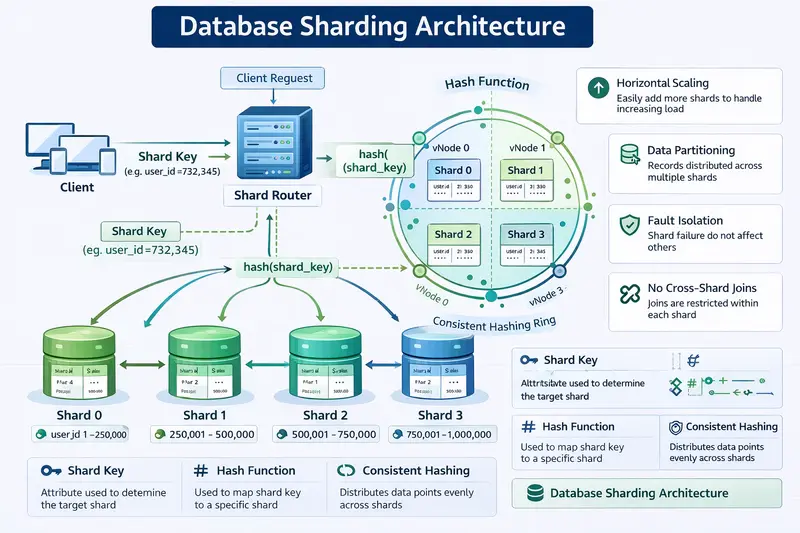
Database Sharding represents a fundamental horizontal scaling technique in system design that divides a single large database into multiple smaller, independent shards. Each shard operates as a complete, self-contained database instance hosted on separate servers or nodes, holding only a specific subset of the overall data. This architectural approach enables distributed databases to handle massive volumes of data and traffic that would overwhelm any single database server.

The core principle of sharding relies on a deliberate data partitioning strategy where the application layer or a dedicated shard router determines which shard should store or retrieve any given record. Unlike vertical scaling, which simply upgrades hardware on one machine, database sharding distributes both storage and compute resources across many machines, delivering linear scalability while maintaining high availability and fault isolation.

Why Organizations Adopt Database Sharding

Modern distributed systems face exponential growth in data and user concurrency. A monolithic database quickly encounters limits in CPU, memory, disk I/O, and network bandwidth. Database sharding addresses these bottlenecks by allowing each shard to process queries independently, reducing contention and eliminating single points of failure.

Sharding also improves read and write performance because queries are routed only to the relevant shard, avoiding full-table scans across the entire dataset. In high-traffic applications such as social platforms, e-commerce marketplaces, or real-time analytics engines, sharding ensures that response times remain predictable even as the user base grows from millions to billions of records.

Core Components of a Sharded Database Architecture

A production-grade sharded database consists of several interconnected layers:

• Shard Key: The critical field or composite value used to route data.
• Shard Router: A middleware component that calculates the target shard for every operation.
• Individual Shards: Independent database instances, each with its own storage engine, indexes, and often its own replication setup.
• Configuration Store: A centralized metadata service that tracks shard mappings and cluster topology.
• Application Clients: Services that interact transparently with the sharded cluster through the router layer.

Each shard typically maintains its own replica set using master-slave replication or multi-master replication to guarantee high availability within the shard itself.

Choosing and Designing the Shard Key

The success of any sharding implementation hinges entirely on the selection of an effective shard key. An ideal shard key must satisfy three non-negotiable properties: high cardinality, even distribution, and alignment with dominant query patterns.

Cardinality ensures enough unique values exist to spread data evenly. Distribution prevents hotspots where one shard receives disproportionately more traffic. Query alignment guarantees that most operations can be satisfied by touching only a single shard, avoiding expensive cross-shard operations.

Common pitfalls include using auto-incrementing integers or timestamps as shard keys, which create range hotspots and force constant resharding. Instead, designers prefer user_id, session_id, geographic_region, or hashed composites that naturally balance load.

Major Sharding Strategies with Complete Implementation Examples

Range-Based Sharding

Range-based sharding assigns entire contiguous ranges of the shard key to specific shards. This strategy excels when applications frequently run range queries such as “find all orders between date X and date Y.”

# Complete Python implementation of a range-based shard router
class RangeShardRouter:
    def __init__(self):
        # Define ranges and their corresponding shard identifiers
        self.ranges = [
            (0, 1000000, 0),      # Shard 0: keys 0 to 999,999
            (1000000, 2000000, 1), # Shard 1: keys 1,000,000 to 1,999,999
            (2000000, float('inf'), 2) # Shard 2: all remaining keys
        ]

    def get_shard(self, shard_key):
        if not isinstance(shard_key, (int, float)):
            raise ValueError("Range sharding requires numeric shard key")

        for start, end, shard_id in self.ranges:
            if start <= shard_key < end:
                return shard_id
        raise ValueError("Shard key out of defined ranges")

# Usage example
router = RangeShardRouter()
print(router.get_shard(1500000))  # Returns 1

While simple, range-based sharding requires careful pre-allocation of ranges and periodic resharding when any range becomes saturated.

Hash-Based Sharding

Hash-based sharding applies a deterministic hash function to the shard key and uses modulo arithmetic to select the target shard. This delivers near-perfect distribution regardless of the original key values.

# Complete Python implementation of hash-based sharding with MD5
import hashlib

class HashShardRouter:
    def __init__(self, num_shards: int):
        if num_shards < 1:
            raise ValueError("Number of shards must be at least 1")
        self.num_shards = num_shards

    def get_shard(self, shard_key: str) -> int:
        # Convert key to string if necessary
        key_str = str(shard_key)
        # Generate 128-bit MD5 hash and convert to integer
        hash_object = hashlib.md5(key_str.encode('utf-8'))
        hash_int = int(hash_object.hexdigest(), 16)
        # Map to shard using modulo
        return hash_int % self.num_shards

# Production-ready usage
router = HashShardRouter(num_shards=8)
print(router.get_shard("user_987654"))  # Returns a consistent shard ID between 0-7

Hash-based sharding virtually eliminates hotspots but makes range queries impossible without scattering requests across all shards.

Consistent Hashing for Dynamic Clusters

Consistent hashing places both shards and data points on a conceptual hash ring, minimizing data movement when shards are added or removed. This strategy is the foundation of many modern distributed databases.

# Complete minimal consistent hashing implementation with virtual nodes
import hashlib
from bisect import bisect_left

class ConsistentHashRouter:
    def __init__(self, nodes: list, virtual_nodes: int = 100):
        self.ring = []
        self.node_map = {}
        self.virtual_nodes = virtual_nodes

        for node in nodes:
            for i in range(self.virtual_nodes):
                virtual_key = f"{node}:{i}"
                hash_val = self._hash(virtual_key)
                self.ring.append(hash_val)
                self.node_map[hash_val] = node
        self.ring.sort()

    def _hash(self, key: str) -> int:
        return int(hashlib.md5(key.encode()).hexdigest(), 16)

    def get_shard(self, shard_key: str) -> str:
        if not self.ring:
            raise ValueError("No nodes in the ring")
        hash_val = self._hash(str(shard_key))
        # Find the first node clockwise on the ring
        idx = bisect_left(self.ring, hash_val)
        if idx == len(self.ring):
            idx = 0
        return self.node_map[self.ring[idx]]

# Example cluster initialization
router = ConsistentHashRouter(nodes=["shard-0", "shard-1", "shard-2"], virtual_nodes=50)
print(router.get_shard("order_abc123"))

When a new shard joins the cluster, only a small fraction of keys are reassigned, preserving overall system stability.

Implementing Sharding at the Application Level

Most sharded systems place routing logic inside the application or a dedicated API gateway rather than inside the database engine. The application extracts the shard key from every request, consults the router, and directs the SQL or NoSQL query exclusively to the responsible shard connection pool.

Database-Level Sharding Solutions

Certain database engines provide native sharding capabilities. MongoDB uses a shard key defined at collection creation and automatically routes operations through mongos query routers. PostgreSQL with the Citus extension converts a standard instance into a distributed database where tables are transparently sharded across worker nodes using the same shard key logic described above.

Critical Challenges and Mitigation Strategies

Cross-shard joins become impossible at the database level. The recommended mitigation is aggressive denormalization so that all data required for a single business operation lives inside one shard. When denormalization is insufficient, applications perform scatter-gather operations: issuing parallel queries to multiple shards and merging results in memory.

Distributed transactions spanning shards require either the two-phase commit protocol or the saga pattern. Both introduce latency and failure complexity, so designers prefer to keep transactions strictly within a single shard.

Resharding and rebalancing demand careful orchestration. Modern systems use background migration jobs that copy data to new shards while maintaining dual writes during the transition, then atomically update routing metadata once migration completes.

Security, Monitoring, and Operational Excellence

Each shard must enforce identical authentication, authorization, and encryption policies. Centralized logging and distributed tracing aggregate metrics across the entire sharded cluster so operators can detect imbalanced load or failing shards instantly. Tools that monitor per-shard query latency, connection counts, and disk usage become essential for maintaining observability.

Advanced Considerations for Production Systems

Read replicas can be added to individual shards for read-heavy workloads without affecting the sharding topology. Geo-sharding places data closer to users by routing based on geographic shard keys, dramatically reducing latency for global applications.

Backup strategies must capture each shard independently while coordinating consistent snapshots across the cluster. Capacity planning involves continuous monitoring of shard utilization to trigger proactive addition of new nodes before any shard approaches saturation.

Database Sharding transforms the way system designers think about scalability. By mastering shard key selection, routing algorithms, consistent hashing, and operational patterns, engineers build systems that gracefully handle billions of records and millions of concurrent users while preserving the simplicity and performance characteristics of a single database.

An image for the reader to understand the article:

System Design Handbook

To deepen your mastery of Database Sharding and every other critical concept in system design, purchase the System Design Handbook today at https://codewithdhanian.gumroad.com/l/ntmcf. It delivers the complete professional reference you need to build production-grade distributed systems.