Demonetization Simulation
Check out this Pen I made!

Check out this Pen I made!
Web Scraping for Beginners: Sell Data as a Service
As a developer, you’re likely aware of the power of web scraping in extracting valuable data from websites. But have you ever considered selling this data as a service? In this article, we’ll walk you through the steps of web scraping for beginners and explore the monetization opportunities that come with it.
Step 1: Choose Your Target Website
The first step in web scraping is to identify the website you want to scrape. This could be a website that provides valuable data such as stock prices, weather forecasts, or social media metrics. For this example, let’s use the website https://www.example.com.
Step 2: Inspect the Website’s HTML Structure
To scrape a website, you need to understand its HTML structure. Use your browser’s developer tools to inspect the website’s HTML elements. Identify the elements that contain the data you want to scrape. For example, if you want to scrape the website’s headings, you would look for <h1>, <h2>, etc. elements.
Step 3: Write Your Web Scraping Code
Now it’s time to write your web scraping code. You can use a programming language like Python or JavaScript to write your scraper. For this example, we’ll use Python with the requests and BeautifulSoup libraries.
import requests
from bs4 import BeautifulSoup

# Send a GET request to the website
url = "https://www.example.com"
response = requests.get(url)

# If the GET request is successful, the status code will be 200
if response.status_code == 200:
    # Get the content of the response
    page_content = response.content

    # Create a BeautifulSoup object and specify the parser
    soup = BeautifulSoup(page_content, 'html.parser')

    # Find all the headings on the webpage
    headings = soup.find_all(['h1', 'h2', 'h3', 'h4', 'h5', 'h6'])

    # Print out the headings
    for heading in headings:
        print(heading.text)
Step 4: Handle Anti-Scraping Measures
Some websites have anti-scraping measures in place to prevent bots from scraping their data. These measures can include CAPTCHAs, rate limiting, and IP blocking. To handle these measures, you can use techniques such as:
python
import requests
from bs4 import BeautifulSoup
import random
import time

# List of user agents
user_agents = [
    'Mozilla/5.0 (Windows NT 10.0; Win64; x64) AppleWebKit/537.36 (KHTML, like Gecko) Chrome/58.0.3029.110 Safari/537.3',
    'Mozilla/5.0 (Windows NT 6.1; WOW64) AppleWebKit/537.36 (KHTML, like Gecko) Chrome/51.0.2704.103 Safari/537.36',
    'Mozilla/5.0 (Windows NT 10.0; Win64; x64; rv:53.0) Gecko/20100101 Firefox/53.0'
]

# Choose a random user agent
user_agent = random.choice(user_agents)

# Send a GET request to the website
url = "https://www.example.com"
headers = {'User-Agent': user_agent}
response = requests.get(url, headers=headers)

# If the GET request is successful, the status code will be 200
if response.status_code == 200:
    # Get the content of the response
    page_content = response.content

    # Create a BeautifulSoup object and specify the
Everyone uses cosine similarity. Tutorials use it. Frameworks default to it. If you ask “which distance metric should I use?”, the answer is always “cosine, probably.”
But here is the thing: your vector database supports other metrics. And those metrics unlock use cases that cosine literally cannot handle.
This is not a math lecture. This is a practical guide. Five metrics, five real-world problems, working code you can run in two minutes. By the end, you will look at your vector database differently.
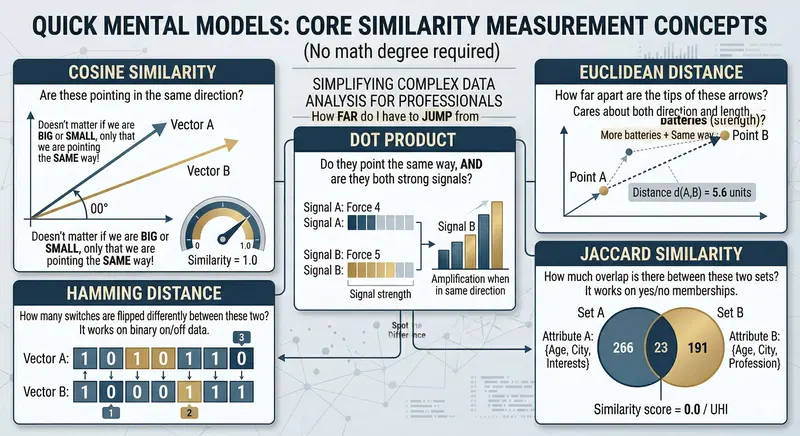
A quick mental model (no math degree required)
Before we dive in, let’s build some intuition. Imagine you have two arrows on a piece of paper:
Cosine asks: “Do these arrows point in the same direction?” It does not care how long they are.
Euclidean asks: “How far apart are the tips of these arrows?” It cares about both direction and length.
Dot Product asks: “Do they point the same way, AND are they both strong signals?” Direction plus intensity.
Hamming asks: “How many switches are flipped differently between these two?” It works on binary on/off data.
Jaccard asks: “How much overlap is there between these two sets?” It works on yes/no memberships.
That is it. Five different questions, five different superpowers. Let’s see them in action.

Setup
pip install velesdb
One line. No Docker. No API keys. VelesDB is an embedded database written in Rust (~6MB binary). It runs in your process.
import velesdb

db = velesdb.Database("./my_data")
1. Cosine: the one you already know (but maybe not why)
The question it answers: “Are these two things about the same topic?”
Cosine measures the angle between two vectors. If two documents are about machine learning, their embedding vectors will point in roughly the same direction, regardless of document length. A 280-character tweet and a 10-page paper about the same topic will score high.
collection = db.create_collection("articles", dimension=4, metric="cosine")

# Simulated embeddings: [tech, science, cooking, sports]
collection.upsert([
    {"id": 1, "vector": [0.9, 0.8, 0.0, 0.0], "payload": {"title": "Introduction to Machine Learning"}},
    {"id": 2, "vector": [0.8, 0.9, 0.0, 0.0], "payload": {"title": "Neural Networks Explained"}},
    {"id": 3, "vector": [0.0, 0.1, 0.9, 0.8], "payload": {"title": "Best Pasta Recipes"}},
    {"id": 4, "vector": [0.1, 0.0, 0.0, 0.9], "payload": {"title": "World Cup 2026 Preview"}},
    {"id": 5, "vector": [0.7, 0.6, 0.0, 0.1], "payload": {"title": "Deep Learning for Beginners"}},
])

results = collection.search(vector=[0.85, 0.75, 0.0, 0.0], top_k=3)
score=1.000  Introduction to Machine Learning
score=0.994  Deep Learning for Beginners
score=0.993  Neural Networks Explained
All three AI articles cluster together. Pasta and football? Nowhere close. This is cosine’s sweet spot: semantic similarity where you care about topic, not intensity.
When to use cosine: semantic search, document similarity, FAQ matching, any text embedding comparison.
2. Euclidean: the anomaly hunter
The question it answers: “How far is this point from what’s normal?”
Here is where it gets interesting. Imagine IoT sensors on a factory floor, each sending readings every minute: temperature, pressure, humidity, vibration. Normal readings cluster in a tight neighborhood. An anomaly is a point that is physically far from the cluster.
Cosine would miss this. Why? Because a reading of [78C, 985hPa, 12%, 4.8g] could point in a similar direction to [22C, 1013hPa, 45%, 0.3g]. Same general “shape” of data, vastly different magnitudes. Cosine says “similar.” Euclidean says “these are 70 units apart, something is on fire.”
collection = db.create_collection("sensors", dimension=4, metric="euclidean")

# Sensor: [temperature_C, pressure_hPa, humidity_%, vibration_g]
collection.upsert([
    {"id": 1, "vector": [22.0, 1013.0, 45.0, 0.3], "payload": {"status": "normal", "time": "08:00"}},
    {"id": 2, "vector": [22.5, 1012.5, 47.0, 0.3], "payload": {"status": "normal", "time": "09:00"}},
    {"id": 3, "vector": [21.8, 1013.5, 44.0, 0.4], "payload": {"status": "normal", "time": "10:00"}},
    {"id": 4, "vector": [23.0, 1012.0, 46.0, 0.3], "payload": {"status": "normal", "time": "11:00"}},
    {"id": 5, "vector": [78.0, 985.0, 12.0, 4.8],  "payload": {"status": "ANOMALY", "time": "11:15"}},
])

results = collection.search(vector=[22.0, 1013.0, 45.0, 0.3], top_k=5)
distance=  0.00  08:00 - normal
distance=  1.14  10:00 - normal
distance=  1.73  11:00 - normal
distance=  2.12  09:00 - normal
distance= 70.92  11:15 - ANOMALY  *** ALERT ***
Normal readings are all within distance 0-2 of each other. The anomaly is at distance 70. That is not a subtle difference. That is a fire alarm.
When to use euclidean: anomaly detection, IoT monitoring, fraud detection, anything where the absolute values matter, not just the direction.
3. Dot Product: the smart recommender
The question it answers: “Is this relevant to me, and how confident are you?”
Dot product is cosine’s bigger sibling. Cosine only looks at direction. Dot product looks at direction AND magnitude. Think of it this way: two movies can both be sci-fi (same direction), but a critically acclaimed blockbuster has a “louder” embedding signal than a forgettable B-movie.
With cosine, they would score equally. With dot product, quality rises to the top.
collection = db.create_collection("movies", dimension=4, metric="dotproduct")

# Dimensions: [sci_fi, action, drama, comedy]
# Higher magnitude = stronger signal / higher quality
collection.upsert([
    {"id": 1, "vector": [0.95, 0.80, 0.30, 0.05], "payload": {"title": "Interstellar", "rating": 8.7}},
    {"id": 2, "vector": [0.40, 0.35, 0.10, 0.02], "payload": {"title": "Low-Budget Sci-Fi B-Movie", "rating": 3.2}},
    {"id": 3, "vector": [0.85, 0.90, 0.20, 0.10], "payload": {"title": "The Matrix", "rating": 8.7}},
    {"id": 4, "vector": [0.05, 0.05, 0.10, 0.95], "payload": {"title": "Comedy Special", "rating": 7.0}},
    {"id": 5, "vector": [0.70, 0.60, 0.50, 0.05], "payload": {"title": "Blade Runner 2049", "rating": 8.0}},
])

results = collection.search(vector=[0.9, 0.8, 0.1, 0.0], top_k=5)
score=1.525  Interstellar (rating: 8.7)
score=1.505  The Matrix (rating: 8.7)
score=1.160  Blade Runner 2049 (rating: 8.0)
score=0.650  Low-Budget Sci-Fi B-Movie (rating: 3.2)
score=0.095  Comedy Special (rating: 7.0)
Notice: the B-movie is sci-fi (same direction as Interstellar), but it ranks way below because its embedding magnitude is weaker. Dot product naturally surfaces quality. This is why recommendation systems at scale often prefer it over cosine.
When to use dot product: recommendation engines, search ranking where content quality matters, any case where you want relevance weighted by confidence.
4. Hamming: the duplicate detective
The question it answers: “How many bits are different between these two?”
This one is completely different from the previous three. Hamming works on binary vectors (0s and 1s) and simply counts how many positions differ. It is lightning fast and perfect for one thing: comparing hashes.
Real-world scenario: you run a content platform. Users upload images. You want to detect reposts, even if someone cropped the image, added a filter, or recompressed it. The approach: compute a perceptual hash (pHash) of each image, which produces a binary fingerprint. Near-duplicate images have fingerprints that differ by just a few bits.
collection = db.create_collection("image_hashes", dimension=16, metric="hamming")

# Simulated 16-bit perceptual hashes
collection.upsert([
    {"id": 1, "vector": [1,0,1,1,0,0,1,0,1,1,0,1,0,0,1,1],
     "payload": {"file": "sunset_original.jpg", "source": "photographer"}},
    {"id": 2, "vector": [1,0,1,1,0,0,1,0,1,1,0,1,0,0,1,0],
     "payload": {"file": "sunset_cropped.jpg", "source": "instagram repost"}},
    {"id": 3, "vector": [1,0,1,1,0,0,1,0,1,1,0,1,0,1,1,1],
     "payload": {"file": "sunset_filtered.jpg", "source": "pinterest"}},
    {"id": 4, "vector": [0,1,0,0,1,1,0,1,0,0,1,0,1,1,0,0],
     "payload": {"file": "cat_photo.jpg", "source": "original"}},
    {"id": 5, "vector": [1,0,1,1,0,0,1,0,1,1,0,1,0,0,0,1],
     "payload": {"file": "sunset_watermarked.jpg", "source": "stock site"}},
])

new_upload = [1,0,1,1,0,0,1,0,1,1,0,1,0,0,1,1]  # same as original
results = collection.search(vector=new_upload, top_k=5)
hamming= 0 bits  [DUPLICATE      ]  sunset_original.jpg (photographer)
hamming= 1 bits  [NEAR-DUPLICATE ]  sunset_cropped.jpg (instagram repost)
hamming= 1 bits  [NEAR-DUPLICATE ]  sunset_filtered.jpg (pinterest)
hamming= 1 bits  [NEAR-DUPLICATE ]  sunset_watermarked.jpg (stock site)
hamming=16 bits  [different image]  cat_photo.jpg (original)
Zero to two bits difference? That is the same image with minor modifications. A content moderation bot can flag these in real-time. No ML model needed. No GPU. Just binary comparison at database speed.
When to use hamming: image deduplication, audio fingerprinting, DNA sequence comparison, binary feature matching, plagiarism detection with locality-sensitive hashing.
5. Jaccard: the taste matcher
The question it answers: “How much overlap is there between these two sets?”
Jaccard is beautifully simple: take two sets, divide the size of their intersection by the size of their union. If you and I both like 3 of the same genres out of 4 total unique genres between us, that is 75% Jaccard similarity.
No embeddings. No ML model. No neural network. Just set math.
collection = db.create_collection("user_profiles", dimension=10, metric="jaccard")

# Genres: [action, comedy, sci-fi, horror, drama, romance, thriller, documentary, anime, musical]
collection.upsert([
    {"id": 1, "vector": [1,0,1,0,1,0,1,0,0,0],
     "payload": {"user": "Alice", "likes": "action, sci-fi, drama, thriller"}},
    {"id": 2, "vector": [0,1,0,0,0,1,0,0,0,1],
     "payload": {"user": "Bob", "likes": "comedy, romance, musical"}},
    {"id": 3, "vector": [1,0,1,1,0,0,1,0,1,0],
     "payload": {"user": "Charlie", "likes": "action, sci-fi, horror, thriller, anime"}},
    {"id": 4, "vector": [1,1,1,1,1,1,1,1,1,1],
     "payload": {"user": "Dave", "likes": "literally everything"}},
    {"id": 5, "vector": [1,0,1,0,0,0,0,1,0,0],
     "payload": {"user": "Eve", "likes": "action, sci-fi, documentary"}},
])

results = collection.search(vector=[1,0,1,0,1,0,0,0,0,0], top_k=5)
75.0% match  Alice (action, sci-fi, drama, thriller)
50.0% match  Eve (action, sci-fi, documentary)
33.3% match  Charlie (action, sci-fi, horror, thriller, anime)
30.0% match  Dave (literally everything)
 0.0% match  Bob (comedy, romance, musical)
Alice shares 3 out of 4 unique genres with you. Dave likes everything, but his union is 10 genres while the overlap is only 3, so Jaccard penalizes him. Bob has zero overlap. The math is transparent, explainable, and instant.
When to use jaccard: user matching, product tagging, skill matching in recruiting, collaborative filtering, any comparison of categorical membership.
The cheat sheet
| Metric | Best for | Score meaning | Think of it as |
|---|---|---|---|
| Cosine | Semantic search | 1.0 = same topic | “Same direction?” |
| Euclidean | Anomaly detection | Lower = closer | “How far apart?” |
| Dot Product | Recommendations | Higher = better match | “Same direction + strong signal?” |
| Hamming | Hash comparison | Lower = more similar | “How many bits differ?” |
| Jaccard | Set overlap | 1.0 = identical sets | “How much in common?” |
The full picture
Choosing the right distance metric is like choosing the right tool. You can hammer a screw into wood, but a screwdriver works better.
Most developers never think about this because most tutorials only show cosine. But the moment you realize that euclidean catches anomalies that cosine misses, or that Jaccard gives you a recommendation engine without any ML, your vector database becomes something much more versatile than a “semantic search box.”
All the code in this article runs as-is. You can grab the complete script from GitHub and try it yourself.
pip install velesdb
python distance_metrics_demo.py
VelesDB is a source-available embedded database (Elastic License 2.0) written in Rust. ~6MB binary, no Docker, no server process, no API keys. Just pip install and go.
Full docs: velesdb.com/en
GitHub: github.com/cyberlife-coder/VelesDB
Python SDK: pypi.org/project/velesdb
What distance metric surprised you the most? Have you used Hamming or Jaccard in a real project? I’d love to hear about it in the comments.
Qdrant is a vector database built for AI applications — semantic search, recommendation systems, and RAG pipelines. REST and gRPC APIs with filtering and payload storage.
Setup
docker run -p 6333:6333 qdrant/qdrant
Create Collection
const response = await fetch('http://localhost:6333/collections/products', {
  method: 'PUT',
  headers: { 'Content-Type': 'application/json' },
  body: JSON.stringify({
    vectors: { size: 384, distance: 'Cosine' }
  })
});
Index Documents with Embeddings
import { QdrantClient } from '@qdrant/js-client-rest';

const client = new QdrantClient({ url: 'http://localhost:6333' });

// Upsert points with vectors and payload
await client.upsert('products', {
  points: [
    {
      id: 1,
      vector: await getEmbedding('Wireless bluetooth headphones with noise cancellation'),
      payload: { name: 'Headphones', price: 89.99, category: 'audio' }
    },
    {
      id: 2,
      vector: await getEmbedding('Mechanical keyboard with Cherry MX switches'),
      payload: { name: 'Keyboard', price: 129.99, category: 'peripherals' }
    }
  ]
});
Semantic Search
const queryVector = await getEmbedding('good headphones for music');

const results = await client.search('products', {
  vector: queryVector,
  limit: 5,
  filter: {
    must: [{ key: 'price', range: { lte: 100 } }]
  },
  with_payload: true
});
// Returns headphones (semantically similar) under $100
Recommendation API
const recommendations = await client.recommend('products', {
  positive: [1, 5],   // IDs user liked
  negative: [3],       // IDs user disliked
  limit: 10,
  filter: { must: [{ key: 'category', match: { value: 'audio' } }] }
});
REST API
# Search
curl -X POST http://localhost:6333/collections/products/points/search
  -d '{"vector":[0.1,0.2,...],"limit":5,"filter":{"must":[{"key":"category","match":{"value":"audio"}}]}}'

# Get collection info
curl http://localhost:6333/collections/products

# Scroll through points
curl -X POST http://localhost:6333/collections/products/points/scroll
  -d '{"limit":10,"with_payload":true}'
Why This Matters
Need custom AI search or vector database tools? I build developer tools. Check out my web scraping actors on Apify or reach out at [email protected] for custom solutions.
Today I worked on a wallet system like GPay or PhonePe, where users can send money to each other. The main focus was Atomicity from ACID properties.
Atomicity means “all or nothing”.
If a transaction fails in between, everything should go back to the original state.
Transaction
I wrote a transaction like this
BEGIN;
UPDATE accounts
SET balance = balance - 200
WHERE name = 'Alice';
UPDATE accounts
SET balance = balance + 200
WHERE name = 'Bob';
COMMIT;
Now Testing Failure
I intentionally broke the second query (credit to Bob).
BEGIN;
UPDATE accounts
SET balance = balance - 200
WHERE name = 'Alice';
UPDATE accounts
SET balancee = balance + 200
WHERE name = 'Bob';
COMMIT;
BEGIN – start transaction
Do all operations
If success – COMMIT
If error – ROLLBACK
Atomicity ensures no partial transactions, which is very important in payment systems.
This is a submission for the Notion MCP Challenge
What I Built
I built Eco-Loom, a multi-facility sustainability operations workspace that helps teams track carbon emissions without drowning in spreadsheets, scattered documents, and disconnected reporting tools.
The idea came from a simple frustration:
carbon accounting is often treated like a reporting exercise at the end of the month—when it should feel like an operational system teams can use every day.
Eco-Loom turns that process into a live workflow.
Teams can:
All from a single workspace.
The product is designed around visibility and action.
Instead of asking:
“Where did this number come from?”
“Which site is off track?”
Eco-Loom makes those answers visible immediately.
🎥 Video Demo
Try it yourself:
Demo Login Credentials:
Video walkthrough:
In the demo, I show how a team can:
💻 Show Us the Code
A key part of the implementation is the company-scoped Notion configuration layer.
Since Eco-Loom is multi-workspace and multi-facility, Notion cannot be treated as a single global integration.
export async function getCompanyNotionConfig(
  companyId: string,
  options: CompanyNotionConfigOptions = {}
) {
  const { createIfMissing = false, adoptLegacy = true } = options;

  const companyConfig = await db.notionConfig.findUnique({
    where: { companyId },
  });

  if (companyConfig) {
    return ensureEncryptedNotionApiKey(companyConfig);
  }

  if (createIfMissing) {
    return db.notionConfig.upsert({
      where: { companyId },
      update: {},
      create: {
        companyId,
        syncEnabled: true,
      },
    });
  }

  return null;
}
That small layer matters because it:
🔗 How I Used Notion MCP
Notion MCP is one of the most important parts of Eco-Loom.
I used it to connect Eco-Loom with structured Notion databases for:
This means Notion is not just a note-taking add-on—it becomes the collaboration layer around the product.
With MCP, Eco-Loom can:
⚙️ What This Unlocks
This creates a much stronger workflow:
All together, they form a closed operational loop.
🚀 Final Thoughts
In short, Notion MCP helped turn Eco-Loom from a dashboard into a true sustainability operating system.
If you’ve ever opened LeetCode, stared at a problem, and immediately closed your laptop — you’re not alone. Grinding algorithm problems in isolation is brutal. No stakes, no community, no reward loop.
That’s why I built Algoora (https://algoora.vercel.app/) — a competitive coding platform designed to be the place you actually want to show up every day.
What Is Algoora?
Algoora is a free web-based competitive coding platform where developers solve algorithmic problems, compete in live tournaments, collaborate with teams, and earn real rewards for their progress. Built for everyone from curious beginners to engineers prepping for FAANG interviews.
Think LeetCode meets a competitive game — with XP, battle passes, cosmetic unlocks, real-time team sessions, and live competitions that make every session feel like it matters.
Core Features
🧩 Problem Library — Solo & Team Modes
Four difficulty tiers: Easy, Medium, Hard, and Extreme. What makes it different is Team Mode — certain problems are designed for two people. One takes the Coder role (writes the solution), the other takes the Explainer role (guides the logic out loud). Real pair programming, built into the platform.
Every problem includes:
⚔️ Live Competitions
Real-time coding tournaments with a live arena, global leaderboard, and time pressure. Race other developers, earn ranking rewards, and get that adrenaline hit of solving a Hard problem with 90 seconds left on the clock.
👥 Teams
Create or join a team, build your roster, and compete together. Teams have dashboards, shared stats, and WebSocket-powered live coding sessions where both teammates see every change in real time.
📈 XP, Levels & Streaks
Every solved problem gives XP. Daily challenges extend your streak. Level up and let your profile show the world how hard you grind.
🏆 Achievements & Badges
A full achievement system — “Solve 100 problems,” “Win your first competition,” “Maintain a 30-day streak.” Badges display publicly on your profile as proof of skill.
🎮 Coding Pass (Battle Pass)
A seasonal battle pass inspired by games like Valorant. Complete challenges, earn XP, unlock cosmetic rewards tier by tier. Premium pass holders get exclusive drops.
🛍️ Shop & Cosmetics
Earn coins by solving problems. Spend them on:
Your profile is your identity — make it yours.
🤖 AI-Powered Error Explanations
When your code fails, the AI doesn’t just show you “Wrong Answer.” It explains why in plain English — what went wrong conceptually and how to think about fixing it. Massive for learners still building their debugging intuition.
🔐 Two-Factor Authentication
TOTP-based 2FA built in. Your account is properly protected.
💎 Free + Premium Tiers
The entire core platform is free. Premium and Elite tiers unlock premium problems and exclusive cosmetics — purchasable with a subscription or with coins you earn in-app.
Who Is Algoora For?
Interview preppers — company tags, editorials, and time/space complexity on every problem.
Competitive programmers — real-time tournaments and global leaderboards.
Developer teams — team coding sessions and collaborative problem solving.
Beginners — hints, AI error explanations, and a gamified progression that makes the learning curve less terrifying.
Anyone who gets bored grinding alone — competitions, streaks, cosmetics, and a battle pass give you reasons to come back every day.
Algoora vs. LeetCode vs. HackerRank
| Feature | Algoora | LeetCode | HackerRank |
|---|---|---|---|
| Live competitions | ✅ | ✅ limited | ✅ |
| Team coding sessions | ✅ | ❌ | ❌ |
| Battle pass / progression | ✅ | ❌ | ❌ |
| Cosmetic customization | ✅ | ❌ | ❌ |
| AI error explanations | ✅ | ❌ | ❌ |
| Earn & spend coins | ✅ | ❌ | ❌ |
| Coder / Explainer roles | ✅ | ❌ | ❌ |
| Free tier | ✅ | ✅ | ✅ |
The Stack
React + TypeScript (Vite) · Tailwind CSS · Node.js · MongoDB · WebSockets · Vercel + Render
Try It Free
No credit card. No friction. Full access to problems, competitions, and team features the moment you sign up.
Why are 80% of engineering organisations abandoning traditional DevOps for Platform Engineering?
The answer starts at Spotify — and it might change how you think about software infrastructure.
The Spotify Origin Story
Around 2018, Spotify faced a critical problem. As they grew from a startup to thousands of engineers, their infrastructure became fragmented. Developers weren’t building features — they were drowning.
Instead of shipping code, engineers spent hours asking:
Context switching and cognitive overload were killing productivity.
The Solution: Backstage
Spotify’s answer was revolutionary: create an abstraction layer on top of all infrastructure tooling.
They called it Backstage — a developer portal powered by a centralised software catalog. One place for everything, accessible to everyone.
Here’s the impact:
But Backstage was just the beginning of something much bigger.
What Exactly Is Platform Engineering?
Think of it as building an Internal Developer Platform (IDP) — a self-service layer that sits between your developers and your infrastructure complexity.
The Three-Layer Architecture
Layer 1: Developer Portal
Your single pane of glass. This is where developers go to discover services, read documentation, and trigger deployments. Tools: Backstage, Port, Cortex.
Layer 2: Service Catalog
The registry of everything. Every API, service, database, and deployment — catalogued and searchable. No more Slack archaeology.
Layer 3: Infrastructure Automation
The magic layer. Using tools like Terraform, Crossplane, or Kratix, you define golden paths — opinionated, pre-approved workflows that let developers deploy without tickets.
DevOps vs Platform Engineering
| Aspect | Traditional DevOps | Platform Engineering |
|---|---|---|
| Who deploys? | Everyone touches infra | Dedicated platform team |
| Self-service | Limited | Full self-service via IDP |
| Cognitive load | High (everyone knows everything) | Low (abstracted complexity) |
| Golden paths | Informal | Codified & enforced |
DevOps said “you build it, you run it.” Platform Engineering says “you build it, we make running it easy.”
The Tools Landscape
Developer Portals
Infrastructure Automation
The Key Insight
These aren’t just pretty UIs — they’re opinionated workflows. The platform team decides the “right way” to deploy, and developers follow golden paths instead of reinventing wheels.
When NOT to Use Platform Engineering
Platform Engineering isn’t a silver bullet.
❌ Skip it if:
✅ Consider it if:
The Numbers
According to Gartner:
Getting Started
Watch the Full Video
I cover all of this in more depth — including architecture diagrams, real-world examples, and the trade-offs nobody talks about:
💬 Have you tried Platform Engineering? What tools are you using? Drop your experience in the comments!
Follow me for more deep dives on software architecture, DevOps evolution, and the tools shaping modern engineering.

“Should we solve this in a meeting?”
Before asking this question, think again.
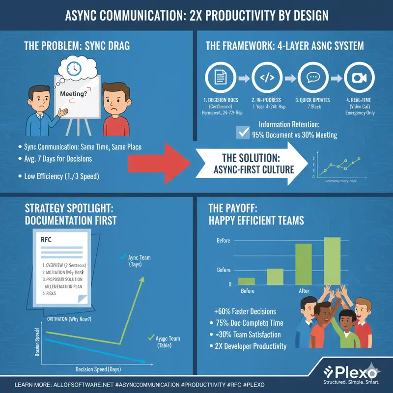
Synchronous communication (meetings): Everyone talks at the same time, same place
Async communication (documents): Each person participates at their own time, their own pace
Productivity difference:
Efficiency increase: 2-3x
At first, meetings seemed faster,
But actually scheduling everyone takes a week.
With async, everyone can participate at their own time, so it’s much faster.
This article covers how to systematically build async communication.
1. Principles of Async Communication
1.1 Core Principles
Principle 1: Documentation First
Sync: Meeting → Unintended decisions → Poor records
Async: Write document → Collect feedback → Perfect records
Principle 2: Capturable
Meeting: What was said vs what's remembered differs
Document: Recorded in clear text
Principle 3: Searchable
Meeting: "Who said this?" → Can't find it
Document: Found immediately via search
1.2 Building Async System
4-Layer Async System:
Information retention rate:
Productivity impact (10-person team, monthly):
2. How to Write Decision Documents
2.1 RFC (Request For Comments) Template
# RFC: Microservices Architecture Migration

## 1. Overview (2 sentences)

We're migrating our monolithic architecture to microservices.
This will increase deployment speed 3x and reduce failure impact.

## 2. Motivation (Why now?)

- Current deployment time: 4 hours (entire team must wait)
- Full system impact when failures occur
- Bottleneck for team expansion

## 3. Proposed Solution

- Current: Monolith
- Proposed: Microservices (3-5 services as macro)

## 4. Alternative Review

| Option             | Pros         | Cons         | Cost |
| ------------------ | ------------ | ------------ | ---- |
| Keep Monolith      | Simple ops   | Hard to scale | Low  |
| Microservices      | High scalability | Complex ops | High |
| Modular Monolith   | Balanced     | Learning curve | Medium |

**Recommendation**: Microservices (high growth expected)

## 5. Implementation Plan

- Phase 1: Infrastructure prep (2 weeks)
- Phase 2: Migrate first microservice (4 weeks)
- Phase 3: Migrate remaining services (8 weeks)

## 6. Risks and Mitigation

| Risk        | Impact | Mitigation      |
| ----------- | ------ | --------------- |
| Deployment failure | High | Blue-green deployment |
| Performance degradation | High | Load testing |
| Team learning curve | Medium | Training program |

## 7. Metrics

- Success metric: Deployment time < 30 min
- Monitoring: Inter-service latency < 100ms
- Failure criteria: Increased failure frequency

## Approval Process

- [ ] Tech team review (by Mon)
- [ ] PM review (by Tue)
- [ ] Executive approval (by Wed)

## Feedback Period

This RFC collects feedback for 5 days (Tue-Sat).
2.2 Decision Record Template
# ADR-001: Select PostgreSQL as Database

## Status: Approved (2025-01-20)

## Problem

Which database should we use?

- Performance: Need high throughput
- Cost: Limited budget
- Team capability: SQL experience available

## Options Considered

### Option 1: PostgreSQL

- Pros: Open source, high stability, low cost
- Cons: Complex horizontal scaling

### Option 2: MongoDB

- Pros: Easy horizontal scaling
- Cons: High cost (cloud), difficult schema management

### Option 3: DynamoDB

- Pros: Fully managed, automatic horizontal scaling
- Cons: High cost, many query constraints

## Decision

**We choose PostgreSQL.**

### Reasons

1. Cost: $5k/year vs MongoDB $15k vs DynamoDB $20k
2. Team capability: Rich SQL experience
3. Performance: Sufficient for expected throughput over next 3 years
4. Horizontal scaling: Read replicas sufficient

## Impact

- Development: Familiar tech → Fast development
- Operations: Increased management responsibility (mitigated by using cloud RDS)
- Cost: $5k saved per year

## Rollback Plan

If need to change to MongoDB:

- Migration cost: $50k
- Migration period: 3 weeks
- Trigger: Exceed throughput (e.g., 100,000 requests/sec)

## Review Schedule

Re-review after 6 months (2025-07-20)
3. Collecting Async Feedback
3.1 Effective Feedback Collection
RFC Feedback Process:
Feedback quality criteria:
Participation activation:
3.2 Writing Feedback Request Messages
Good example:
Please provide feedback on this technology selection RFC.
Especially looking for feedback from these perspectives:

1. Dev team: Implementation difficulty, required tech training
2. Ops team: Operational complexity, monitoring approach
3. PM: Schedule impact, cost
4. Security: Security impact

Feedback submission deadline: Thursday 17:00
Bad example:
Please give feedback.
4. Utilizing Async Tools
4.1 Optimal Use by Tool
Major async tools:
Tool selection by scenario:
5. Meeting Elimination Strategy
5.1 Meeting → Async Transition
Before (Sync):
Mon-Fri: 15 meetings/week per team
Time: 20 hours/week
Efficiency: 30% (3 day delay)

After (Async):
Mon-Fri: RFC-based decisions
Time: 5 hours/week (only urgent sync)
Efficiency: 85% (decision within 24 hours)

Effect:
- Time: 75% saved
- Efficiency: 180% improvement (3x faster)
- Documentation: 100% vs 30%
5.2 Transition Process
Week 1-2: Introduce "Async-First" policy
- All decisions via document-based RFC
- Meetings only for "urgent" or "complex discussion"
- Train all team members

Week 3-4: Pilot operation
- Convert some meetings to async
- Identify issues and improve

Week 5+: Company-wide expansion
- Async culture established
6. Challenges of Async Communication
6.1 Potential Problems and Solutions
Major challenges and solutions:
Async-First Policy:
7. Measurement and Improvement
Async communication effectiveness measurement:
Key Summary
By introducing async communication:
Achieving 2x productivity = 2x developer capability
Start today:
Small changes make a big difference.
Need async-friendly project management with AI-powered task breakdown? Check out Plexo.
AI-Driven Code Review: How I Reduced Bug Rate by 65%
Code review is broken.
We spend hours staring at PRs, catching the same bugs over and over. We miss critical issues because we’re tired or distracted. We delay releases because reviews take too long.
I know this because I lived it.
For 90 days, I tracked every code review I did. The data was sobering:
Then I implemented AI-driven code review. The results:
Here’s exactly how I did it.
The Problem: Why Code Review Fails
1. Human Limitations
We’re not machines. We get tired. We get distracted. We miss things.
The data:
2. Inconsistency
Different reviewers catch different things. Style guides help, but they’re not enough.
The data:
3. Scale Issues
As teams grow, reviews get slower. More code, more reviewers, more delays.
The data:
The Solution: AI-Driven Code Review
I implemented a 3-layer AI review system:
Layer 1: Pre-Review Analysis
Tool: Custom AI Scripts + Static Analysis
Before a human ever sees the PR, AI analyzes it:
Results:
Layer 2: AI-Assisted Human Review
Tool: GitHub Copilot + Custom Prompts
When humans review, AI assists:
Results:
Layer 3: Post-Review Learning
Tool: AI Analytics + Feedback Loop
After reviews, AI learns:
Results:
The 14-Day Implementation Plan
Days 1-3: Setup and Baseline
Day 1: Measure Your Current State
Day 2: Choose Your Tools
Day 3: Set Up Pre-Review Analysis
Days 4-7: Implement AI-Assisted Review
Day 4: Create Review Templates
Day 5: Train Your Team
Day 6: Pilot with One Team
Day 7: Review and Adjust
Days 8-14: Rollout and Optimize
Day 8-10: Gradual Rollout
Day 11-13: Optimize and Scale
Day 14: Measure and Celebrate
The Tools I Use
| Layer | Tool | Cost | Setup Time |
|---|---|---|---|
| Pre-Review | SonarQube | Free | 2 hours |
| Pre-Review | Custom AI Scripts | $20/mo | 4 hours |
| AI-Assisted | GitHub Copilot | $10/mo | 1 hour |
| Post-Review | Custom Analytics | $10/mo | 6 hours |
Total setup time: 13 hours
Total monthly cost: $40
ROI: 50x (based on time saved)
The Metrics That Matter
Before AI-Driven Review
After AI-Driven Review
Financial Impact
Common Pitfalls to Avoid
1. Over-Relying on AI
AI makes mistakes. Always review AI suggestions.
Rule of thumb: Trust AI for 80% of issues, verify the other 20%.
2. Ignoring Team Feedback
Your team knows your codebase better than any AI.
Best practice: Let reviewers override AI suggestions.
3. Not Customizing for Your Context
Generic AI prompts won’t work for every team.
Best practice: Customize prompts for your coding style and patterns.
4. Forgetting About Security
AI might miss security issues.
Best practice: Always run security scans separately.
The Results
After 90 days of using AI-driven code review:
Quality Improvements
Efficiency Improvements
Team Improvements
Business Impact
Your Turn
You don’t need to be an AI expert. You don’t need a huge budget. You just need to start.
Pick one layer of AI-driven review. Implement it this week.
Then come back and tell me how much time you saved.
Resources
Affiliate Disclosure: Some links below are affiliate links. If you purchase through these links, I may earn a commission at no extra cost to you.
Want to learn more? Check out my other articles on AI-powered development workflows.
Have questions? Drop them in the comments below. I reply to every comment.