I can now replay any AI agent stream from production. Here’s how.

I can now replay any AI agent stream from production.

Here’s how.
In my last post, I wrote about the four SSE bugs that break AI agent UIs at 2am — chunk boundary splits, missing token batching, hanging done states, and retry logic that retries the wrong things.

There’s a fifth problem I didn’t cover, because the fix didn’t exist yet.

What do you do the morning after something broke?

The stream is gone. The event sequence that caused the bug evaporated the moment the connection closed. You have a user complaint, maybe a generic error log, and zero ability to reproduce the issue locally because local dev doesn’t have real network conditions, real token rates, or the specific sequence of tool calls that triggered the failure.

Today I shipped AgentStreamRecorder to the agent-stream library to solve exactly this.

The debugging gap nobody talks about
When a REST API fails, you have the request and response in your logs. You can replay it with curl. You can write a regression test. The failure is reproducible.

When an AI agent stream fails mid-flight, you have nothing. The SSE connection is stateful and ephemeral. The events exist in a buffer, get consumed by the client, and are gone. If the frontend shows wrong state — tools that didn’t clear, progress that froze at 60%, text that truncated — you’re debugging from memory and screenshots.

We hit this at Praxiom repeatedly while building 36 production agent tools. The failure pattern was always the same:

  1. User reports the stream “felt wrong” or the UI got stuck
  2. You try to reproduce — works fine in dev
  3. You add more logging — doesn’t help, the issue is in the event sequence, not individual events
  4. You fix something and hope — no regression test possible
  5. Issue reappears three weeks later in a different context
  6. The root problem: we had full observability on every other layer of the stack except the stream itself.

What AgentStreamRecorder does
It’s a drop-in async wrapper. You add two lines to your existing endpoint and every stream gets saved to a .jsonl file automatically.

Before:

@app.post("/chat")
async def chat(req: ChatRequest):
    return agent_stream_response(run_agent(req.message))

After:

from agent_stream.recorder import AgentStreamRecorder

recorder = AgentStreamRecorder("streams/production.jsonl")

@app.post("/chat")
async def chat(req: ChatRequest):
    async def generate():
        async for sse_str in recorder.record(run_agent(req.message)):
            yield sse_str  # passes through unchanged

    return agent_stream_response(generate())

That’s it. The recorder wraps the async generator, tees each SSE event to the file, and re-yields the string unchanged. Your StreamingResponse sees nothing different. The client sees nothing different. Zero impact on latency.

What gets recorded
Each session in the .jsonl file starts with a header line, then one line per event:

{% embed {"session": "f3a2c1b0-...", "started_at": "2026-03-31T02:14:00+00:00", "t": 0}
{"t": 0.0,   "event": "token",      "data": {"text": "Hello, here"}}
{"t": 0.041, "event": "token",      "data": {"text": " is what I found"}}
{"t": 0.052, "event": "tool_use",   "data": {"tool_name": "web_search", "status": "running"}}
{"t": 0.894, "event": "tool_result","data": {"tool_name": "web_search", "duration_ms": 842, "status": "done"}}
{"t": 1.204, "event": "done",       "data": {"num_turns": 1, "tool_count": 1, "duration_ms": 1204}} %}

The t field is seconds since stream start — relative, not absolute — so files are portable across machines and time zones. The format is append-safe: each new session appends to the file with its own UUID and t=0 baseline, so you can keep one file per day and scan it with grep.

Three design decisions worth explaining:

.jsonl not binary. You can grep it. grep ‘”event”: “error”‘ production.jsonl instantly shows every stream that hit an error event, with timing. Binary formats are faster to write but terrible to investigate.

Relative timestamps. Absolute wall-clock timestamps tell you when something happened. Relative timestamps tell you how long it took. Relative is almost always what you need for debugging — “tool_result came back 842ms after tool_use” is more useful than two UTC timestamps you have to subtract.

Flush after every write. The file is flushed after every line, not buffered. If the process crashes mid-stream, you still have everything up to the last event. This matters — crashes are exactly when you most need the recording.

Replaying it
The agent-stream CLI (installed with the package) plays back recordings:

What sessions are in this file?

agent-stream replay production.jsonl –list

The output is valid SSE piped to stdout. You can pipe it to a local dev server, feed it into a test harness, or just watch it in the terminal to see exactly what the client received.

The use case that made this necessary
Here’s the specific failure pattern that pushed us to build this. We had a multi-turn agent that called several tools in sequence. In production with certain inputs, the activeTools array in the React hook wasn’t clearing properly — a tool would finish but its name would stay in the “currently running” UI indefinitely.

Couldn’t reproduce it locally. The tool sequence was always different. Adding console logs to the hook showed correct state at each individual event, but the sequence mattered.

With AgentStreamRecorder, we recorded the failing session from production, replayed it through a local frontend, and watched the hook state update in real-time. Spotted the issue immediately: a tool_result event was arriving before the matching tool_use in one specific sequence, because two tools were running in parallel and the faster one resolved first. The hook was looking for tool names in order; the order wasn’t guaranteed.

Fifteen-minute fix. Would have taken days without the recording.

The bigger pattern: AI agents need a different kind of observability
Standard application observability — request logs, error rates, latency percentiles — doesn’t map cleanly onto AI agent streams. The unit of interest isn’t a request, it’s a session. The signal isn’t an error code, it’s an event sequence. The failure mode isn’t a stack trace, it’s a state machine reaching an unexpected state.

AgentStreamRecorder is a small step toward stream-native observability. Each .jsonl session is a complete, replayable trace of exactly what the agent did and how long each step took. You can diff two sessions to understand why one succeeded and one failed. You can build a test suite from real production recordings. You can grep across thousands of sessions to understand behavioral patterns at scale.

None of this is revolutionary. It’s the kind of thing you’d take for granted in any mature system — request tracing, structured logging, replay-from-log. We just haven’t had it for agent streams.

Getting it
pip install agent-event-stream
from agent_stream.recorder import AgentStreamRecorder

Full source, spec, and React client hook at github.com/abhichat85/agent-stream.

Extracted from Praxiom — Product Intelligence that compounds. Think Cursor for Product Managers.

OpenAI Codex Had a Command Injection Bug That Could Steal Your GitHub Tokens

BeyondTrust’s Phantom Labs just published a report on a command injection vulnerability in OpenAI’s Codex. It’s patched now, but the attack pattern matters because it’s exactly the kind of thing vibe coders won’t see coming.

What Happened

Codex runs tasks inside managed containers that clone your GitHub repo and authenticate using short-lived OAuth tokens. The vulnerability: branch names weren’t sanitized before being passed to shell commands during environment setup.

An attacker could craft a malicious branch name that injects arbitrary shell commands. Those commands execute inside the container with access to your GitHub token.

The attack worked across:

  • The Codex web interface
  • The CLI
  • The SDK
  • IDE integrations

Worse: it could be scaled. Embed a malicious payload in a branch name, and every developer who interacts with that repo through Codex gets compromised.

What Could Be Stolen

The GitHub OAuth tokens Codex uses aren’t just read tokens. In enterprise environments where Codex has broad permissions:

  • Full read/write access to repositories
  • Workflow trigger permissions (CI/CD pipelines)
  • Organization-level access depending on token scope

One compromised branch name. Every Codex user on the repo exposed.

Why This Matters for Vibe Coders

This vulnerability was found by professional security researchers at BeyondTrust. Most vibe coders:

  1. Don’t review branch names for injection payloads
  2. Don’t audit what permissions their AI coding tools have
  3. Don’t know what an OAuth token scope even is
  4. Trust that “it’s a managed container” means it’s safe

The attack surface isn’t your code. It’s your tools.

The Bigger Picture

This dropped the same day Claude Code launched Computer Use (mouse and keyboard control). Two separate stories, same lesson:

AI coding agents are live execution environments with access to your credentials.

They’re not just autocomplete. They run commands, clone repos, access tokens, and now control your screen. Every new capability is a new attack surface.

In the last 7 days:

  • LiteLLM supply chain attack hit 95M monthly downloads (TeamPCP campaign)
  • Same attacker compromised Trivy (vulnerability scanner) and KICS (IaC analyzer)
  • OpenAI Codex command injection exposed GitHub tokens
  • Claude Code gained mouse and keyboard access

The tools we trust to write and test our code are becoming the primary attack vector.

What To Do

  1. Audit your AI tool permissions. What repos can Codex access? What scope do the tokens have? Minimize to read-only where possible.
  2. Pin your dependencies. TeamPCP compromised packages that millions install without version pinning.
  3. Don’t trust container isolation alone. The Codex containers had network access. “Managed” doesn’t mean “secure.”
  4. Scan your deployed apps. If you built it with AI tools, scan it before users find what you missed. VibeCheck is free.
  5. Check for exposed secrets. Branch names, commit messages, config files. AI tools don’t flag these by default.

OpenAI patched this one. The next vulnerability in the next AI coding tool hasn’t been found yet.

Building VibeCheck, a free security scanner for vibe-coded apps. Follow @solobillionsHQ for daily vibe coding security updates.

What Actually Happens When You Leave an ESP32 Running 24/7

There is a small board on a shelf that never sleeps.

No fan noise. No screen. Just a faint warmth if you press a finger against it long enough. The LED stopped blinking weeks ago. Or maybe it still is, and you stopped noticing.

It’s still running.

And that’s where people get it wrong.

They think “running” means stable. Predictable.
Done.

It doesn’t.

It Doesn’t Stay the Same Device

The first version of your ESP32 is the one you flashed. Clean. Intentional. Every line of code accounted for.

That version doesn’t last.

Over time, the device drifts. Not in some mystical sense. In a very literal accumulation of state. Buffers fill and empty. Memory fragments. WiFi reconnects hundreds of times. Timers tick past thresholds you never tested. Edge cases stop being edge cases because given enough hours, everything happens.

You wrote logic assuming a day. Maybe a week.
Leave it for a month and you’re no longer running your code. You’re running everything your code didn’t anticipate.

There’s a difference.

Memory Starts to Behave Like a Surface, Not a Container

On paper, the ESP32 has enough RAM for most lightweight systems. In practice, that RAM becomes uneven over time.

Heap fragmentation is the quiet one. It doesn’t crash immediately. It just reshapes what’s available. Allocations that worked on day one start failing in strange ways. Not clean failures either. Partial allocations. Corrupted data.

Functions returning values that feel slightly off.
You restart the device and everything looks fine again.

That should bother you.

Because it means the system only works in a freshly initialized state. Which means it’s not stable. It’s just temporarily aligned.

Long-running devices expose this quickly.

Especially if you’re doing dynamic allocation, string operations, or anything involving WiFi stacks and JSON parsing.

It’s not dramatic. It’s worse than that. It’s subtle.

WiFi Becomes a Personality Problem

WiFi on the ESP32 is good. Until it isn’t.

When you leave a device running continuously, you start to see patterns that don’t show up in short sessions. Networks drop for a few seconds. Routers rotate channels. DHCP leases expire. Signal strength shifts based on time of day, interference, other devices.

Your ESP32 has to live through all of that.

And most sketches don’t handle it properly.

They check WiFi.status() and reconnect. That’s not enough. Sometimes the stack thinks it’s connected when it isn’t. Sometimes reconnect loops lock up other tasks. Sometimes the device enters a state where it’s technically online but functionally dead. No data moves.

You won’t notice unless you’re logging externally.
From the outside, it looks fine. The LED is still on.

Inside, it’s stalled.

Heat Is Low, But Not Zero

People treat the ESP32 like it’s immune to heat because it runs cool.

That’s only half true.

Yes, it won’t burn your fingers. But over long durations, even small thermal fluctuations matter. Especially if the board is enclosed, or sitting near other electronics, or powered through questionable regulators.

Temperature affects timing. Stability. RF performance.

Not enough to break things instantly. Enough to shift behavior over time.

You start seeing weird resets. Slight timing drift. Sensor readings that slowly diverge.

Nothing obvious. Just enough to make you doubt your data.

Power Quality Starts to Matter More Than Code

For short runs, almost any USB cable and power source will do.

For 24/7 operation, power becomes the foundation.
Cheap adapters introduce ripple. Long cables drop voltage. Sudden load spikes from WiFi transmissions can dip the supply just enough to trigger brownouts.

The ESP32 has brownout detection, but many people disable it when it becomes annoying during development.

That decision comes back later.

Now instead of clean resets, you get undefined behavior. Partial execution. Corrupted state.
A device that “runs fine” for hours suddenly locks up after three days.

You blame the code. It might not be the code.

Time Stops Being Abstract

Most hobby projects ignore time beyond millis().
Leave something running for weeks and time becomes a real dependency.

Timers overflow. Scheduling drifts. Events that rely on precise intervals begin to slide. If you’re syncing with external systems, even small inaccuracies compound.

Without NTP or some form of correction, your device’s sense of time slowly diverges from reality.

At first it’s seconds. Then minutes.

Then your logs stop lining up with anything else.
If your system depends on ordering events, that’s not a minor issue.

Logging Becomes the Only Truth

When a device runs continuously, you stop being present for most of its behavior.

That means your understanding is only as good as your logs.

And most ESP32 setups barely log anything.

A few serial prints during development. Maybe some debug output. Then it gets removed to “clean things up.”

Now something goes wrong at hour 72 and you have no record of what led to it.

You’re blind.

Real 24/7 systems treat logging as a core feature, not an afterthought. Even if it’s just rotating logs on an SD card or pushing minimal telemetry to a server.

Without that, you’re guessing.

And guessing feels a lot like debugging until it doesn’t.

The Device Starts Interacting With the Real World

This is the part people underestimate.

A continuously running ESP32 stops being a test object and becomes part of an environment.

It interacts with networks that change. Power that fluctuates. Inputs that aren’t controlled. People who don’t know it exists.

Maybe it’s scanning RFID tags. Maybe it’s reading sensors. Maybe it’s acting as a node in something larger.

Over time, it accumulates context.

Patterns emerge. Not in a clean dataset sense. In a messy, lived-in way. Missed reads. Duplicate events. Noise that wasn’t present during testing.
You start realizing your logic was built for a lab, not for reality.

And reality is not consistent.

Stability Is Engineered, Not Implied

Leaving an ESP32 running 24/7 doesn’t automatically make it stable.

It reveals whether it is.

Most setups fail this test in quiet ways. Not explosions. Not obvious crashes. Just gradual degradation. A system that becomes less correct over time.

To counter that, you have to design for longevity from the start.

Not complicated changes. Just intentional ones:

  • Watchdogs that actually reset the system when it stalls
  • Periodic soft reboots to clear state
  • Defensive memory handling instead of optimistic allocation
  • Real reconnection logic for WiFi, not just retries
  • External logging so you can see what happened when you weren’t there

None of this is glamorous.
But it’s the difference between a project and a system.

It Becomes Something You Don’t Fully Control

There’s a point where a long-running device stops feeling like a tool and starts feeling like a process.

It runs whether you check it or not. It fails in ways you didn’t directly cause. It recovers sometimes. Other times it doesn’t.

You can tighten it. Monitor it. Reset it.

But you don’t sit inside every execution path anymore.

That distance matters.

Because it forces you to think differently. Less about writing code that works now. More about writing code that survives being left alone.

The Quiet Shift

If you’ve only ever powered your ESP32 during active sessions, you’re seeing a curated version of it.

Clean boots. Short timelines. Controlled inputs.
Leave it running for weeks and you get the unfiltered version.

Not broken. Just honest.

It shows you where your assumptions were thin. Where your system depends on luck. Where stability was implied instead of built.

Most people don’t run their devices long enough to see this.

Which is why their projects feel solid.
Until they aren’t.

Feel like supporting the publication? Look no further than my curated guides on cybersecurity, diy electronics, and more on my gumroad. The guides below pair very well with the content of this post, and these guides are currently keeping me “fed ‘n’ bed” as I am currently in a unique and challenging situation in my life. Any support means the world, and includes lifetime updates and access to my personal email for debugging/discourse. Thanks again, if you read this far- you are obviously on the same wavelength. Keep pushing. 

The BadUSB Factory: Convert Any Flash Drive Into a Weapon

The Ultimate Arduino Project Compendium

Google Calendar — Day View

Google Calendar — Day View

Frontend / Backend Split: 40% Backend · 60% Frontend
Google Calendar Day View is frontend-heavy — but the backend is non-trivial. The frontend solves: virtual scrolling a 24-hour grid, drag-and-drop with snapping, overlapping event layout (interval partitioning), and RRULE expansion. The backend solves: ACID event storage, conflict resolution for concurrent edits, and fan-out notifications to shared calendar members. Both sections get full coverage.

1. Problem + Scope

Design the Google Calendar Day View — a time-grid UI that displays all events for a single day, supports creating/editing/deleting events via drag, resize, and click, handles recurring events, and broadcasts real-time updates to shared-calendar collaborators.

In scope: Day view grid, event CRUD, drag & resize, recurring events (RRULE), overlapping event layout, real-time collaboration on shared calendars, all-day events, timezone rendering.

Out of scope: Meeting Room booking, Google Meet integration, calendar migration/import, Google Tasks integration.

2. Assumptions & Scale

Metric Value
Daily Active Users 500M
Avg events visible in day view 10–20 per user
Peak concurrent users 50M
Event reads (day view load) 3–5 API calls
Peak event writes 10M updates/min → ~167K writes/sec
Event storage per user/year ~10K events × 1KB = 10MB
Total storage 500M × 10MB = 5PB
WebSocket connections (shared calendars) ~5M concurrent

Scale calculation for write path:

167K writes/sec is easily handled by a PostgreSQL cluster with read replicas. No NoSQL needed — events are relational (attendees, calendars, permissions). The fan-out to collaborators (shared calendar update → notify N users) is the harder problem at scale.

These numbers drive the following decisions: PostgreSQL for ACID event storage, Redis for WebSocket session routing, Kafka for fan-out notifications to shared calendar members.

3. Functional Requirements

  • Display a 24-hour time grid for a selected date, showing all events for the user
  • Create events via click-and-drag on the grid
  • Edit events: drag to move (reschedule), drag edge to resize (change duration)
  • Delete events
  • Handle overlapping events — render them side-by-side without overlap
  • Support recurring events defined by RRULE (daily, weekly, monthly, custom)
  • Show all-day events in a dedicated strip at the top
  • Render events from multiple calendars with color coding
  • Real-time sync: if a collaborator edits a shared event, the other user’s view updates within 1 second
  • Timezone-aware: store in UTC, render in the user’s local timezone

4. Non-Functional Requirements

Requirement Target
Initial load latency < 500ms (events visible)
Drag & resize frame rate 60 fps (no jank)
Real-time update latency < 1 second for shared calendars
Availability 99.9%
Consistency Eventual for real-time; strong for event creation/deletion
Offline Read-only view from local cache; writes queued

Consistency model:

Domain Model Justification
Event CRUD Strong (PostgreSQL) Prevents double-booking, attendee confusion
Real-time collaboration Eventual (WebSocket + Kafka) 1-second delay acceptable; last-write-wins
RRULE expansion Computed on read Recurrences are derived — no consistency issue

🧠 Mental Model

Google Calendar Day View has three core flows:

  1. Load flow — user navigates to a date → client fetches events for that day → frontend computes the layout (overlaps, positions, widths) → renders the grid
  2. Edit flow — user drags/resizes/clicks → optimistic UI update locally → API call → server persists → WebSocket broadcasts change to collaborators
  3. Real-time flow — collaborator edits a shared event → Event Service writes to DB → Kafka message → Notification Service → WebSocket push → all connected clients for that calendar receive the update
User navigates to Day View
         │
         ▼
   Fetch /events?date=X
         │
    ┌────┴────────────────────────────┐
    │  LAYOUT ENGINE (client-side)    │
    │  1. Sort events by start time   │
    │  2. Detect overlapping groups   │
    │  3. Assign columns + widths     │
    └────┬────────────────────────────┘
         │
         ▼
   Render 24h grid with positioned events
         │
    User drags event
         │
    ┌────┴──────────────────────────────┐
    │  DRAG ENGINE                      │
    │  1. Snap to 15-min increments     │
    │  2. Optimistic update (local)     │
    │  3. PATCH /events/:id on drop     │
    │  4. WS broadcast to collaborators │
    └───────────────────────────────────┘

⚡ Core Design Principles

Path Optimized For Mechanism
Fast Path Perceived latency Optimistic UI — event moves instantly on drag; API fires async
Reliable Path Correctness If PATCH fails, revert optimistic update + show error toast

5. API Design

Calendar APIs

Method Path Description
GET /api/v1/events?calendarId=&start=&end= Fetch events for a date range. Returns expanded recurrences.
POST /api/v1/events Create event. Returns event with server-assigned ID (idempotency key in body).
PATCH /api/v1/events/:id Partial update — move/resize uses this. Supports start, end, recurrenceAction.
DELETE /api/v1/events/:id?recurrenceAction= Delete single instance or all/future recurrences.
GET /api/v1/calendars List user’s calendars (own + shared). Used to set color coding.

WebSocket

Event Direction Payload
calendar.event.updated Server → Client { eventId, calendarId, changes, updatedBy }
calendar.event.deleted Server → Client { eventId, calendarId, recurrenceAction }

[!TIP]
Interview tip: The recurrenceAction parameter on PATCH/DELETE is a key design question. Options: THIS (only this instance), THIS_AND_FOLLOWING, ALL. Say: “I expose this as a query parameter because the semantic differs from a normal update — it’s modifying the RRULE or creating an exception, not just patching data.”

6. End-to-End Flow

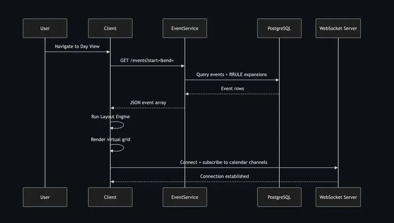
6.1 Day View Load

  1. User navigates to Day View for date 2025-03-28.
  2. Client sends GET /api/v1/events?calendarId=primary&start=2025-03-28T00:00Z&end=2025-03-28T23:59Z.
  3. Event Service queries PostgreSQL: fetch base events + any RRULE exceptions that fall on this date. For each recurring event, expand the RRULE server-side and return the occurrence for this day as a concrete event object.
  4. Response arrives (≤ 500ms). Client receives array of event objects, each with id, start, end, title, calendarId.
  5. Layout Engine runs: sorts events by start time → groups overlapping events → assigns each event a column index and a width fraction. A group of 3 overlapping events each gets width = 1/3 of the slot.
  6. Virtual scroll renders only the visible portion of the 24h grid. Events are positioned absolutely using top = (startMinutes / 1440) * gridHeight and height = (durationMinutes / 1440) * gridHeight.
  7. WebSocket connection opens to wss://calendar.google.com/ws?calendarId=primary. Client subscribes to shared calendars.

6.2 Drag & Drop (Move Event)

  1. User starts dragging an event. Client immediately applies optimistic update: the event visually follows the cursor. The original time is saved in memory for rollback.
  2. As the event moves, client snaps the top position to the nearest 15-minute increment (every gridHeight / 96 pixels).
  3. On drag end, client computes the new start/end from the final Y position.
  4. Client sends PATCH /api/v1/events/:id with { start: newStart, end: newEnd }.
  5. Event Service writes to PostgreSQL. If the event is a recurring instance and recurrenceAction=THIS, it creates an exception record (stores the modified occurrence, marks the RRULE to skip this date).
  6. Event Service publishes calendar.event.updated to Kafka topic calendar-events.
  7. Notification Service consumes from Kafka, looks up all WebSocket connections subscribed to this calendarId, and pushes the update.
  8. All collaborators’ clients receive the WS event and re-render the event at the new time.
  9. If PATCH fails (network error, conflict): client reverts optimistic update, shows error toast, event snaps back to original position.

6.3 🔄 Complete Lifecycle: Load → Layout → Render → Interact → Sync → Re-render

This is the full end-to-end picture — every phase a request passes through from the moment a user opens the day view to the moment a collaborator sees the update.

  1. Load — User navigates to a date. Client fires GET /events?start=&end=. Event Service queries PostgreSQL, expands RRULE occurrences for this day, returns JSON array.
  2. Layout — Client runs the interval partitioning algorithm: sort → group overlapping events → assign columns → compute width fractions. Pure CPU, no network.
  3. Render — Virtual scroll activates. Only the visible hour range is rendered as DOM nodes. Events are positioned absolutely: top = (startMin/1440) * gridH, height = (durationMin/1440) * gridH.
  4. Interact — User drags an event. DOM mutation (no React re-render) moves the event at 60fps. On drop: snap to nearest 15-min grid, compute new time, fire PATCH /events/:id optimistically.
  5. Sync — Event Service writes to PostgreSQL, publishes calendar.event.updated to Kafka. Notification Service consumes, looks up WebSocket connections for all calendarId subscribers in Redis, pushes the update.
  6. Re-render — Every collaborator’s client receives the WS push. Client patches its local event array with the change, re-runs layout for the affected time slot, and re-renders the moved event at the new position.

[!IMPORTANT]
The cycle is: Load once → Layout locally → Render virtually → Interact optimistically → Sync async → Re-render incrementally. No full page reload at any step. Each phase is independent and can fail gracefully without breaking the others.

7. High-Level Architecture

Simple Design

Evolved Design (with Real-Time + Scale)

[!NOTE]
Key Insight: The WebSocket server is stateless fanout — it doesn’t store event data. Kafka decouples write path from notification path. Event Service never directly calls WebSocket servers.

8. Data Model

Entity Storage Key Columns Why this store
Event PostgreSQL event_id, calendar_id, owner_id, title, start_utc, end_utc, rrule, is_all_day ACID — prevents double-booking; relational joins for attendees
Recurrence Exception PostgreSQL event_id, original_date, new_start_utc, new_end_utc, is_deleted Models RRULE overrides without duplicating base event
Calendar PostgreSQL calendar_id, owner_id, name, color, timezone Relational — permissions, sharing, color metadata
Calendar Members PostgreSQL calendar_id, user_id, role (owner/editor/viewer) Many-to-many sharing; permission checks at write time
WS Session Map Redis calendarId → [connectionId, ...] Ephemeral; TTL = connection lifetime. DB lookup = too slow for fanout
Calendar Metadata Cache Redis userId:calendars → JSON TTL = 5min. Avoids DB hit on every day view load

[!NOTE]
Key Insight: Recurring events are stored as a rule + exceptions model (not pre-expanded rows). Expansion happens at read time. Pre-expanding 10 years of weekly events = 520 rows per event × 500M users = storage explosion.

9. Deep Dives

9.1 🧠 Layout Algorithm — Interval Partitioning Problem

Here’s the problem we’re solving: Multiple events on the same day can have overlapping time ranges. Rendering them stacked (one behind the other) makes them unreadable. We need an algorithm that places overlapping events side-by-side with correct widths so all are visible simultaneously.

This is a classic interval partitioning problem — the same problem as scheduling jobs on the minimum number of machines such that no two overlapping jobs share a machine. The minimum number of machines needed = the maximum number of events overlapping at any single point in time.

Naive solution: Render each event at full width. Overlapping events cover each other — user can’t see or click the hidden events.

🧠 Layout Algorithm (Core) — 4 Steps:

Step 1 — Sort events by start time
Sort all events for the day by start_utc ascending. This ensures we process events in chronological order and can greedily assign columns.

Step 2 — Group overlapping events
Scan the sorted list. Maintain a running groupEndTime = max end time seen so far. If the next event’s start < groupEndTime, it belongs to the current overlapping group. When start >= groupEndTime, the current group is complete — finalize widths and start a new group.

Step 3 — Assign columns
Within each overlapping group: maintain an array of columns, each tracking the latest end_time of the event placed there. For each event, find the first column where column.endTime <= event.startTime. Place the event there and update the column’s end time. If no column fits, add a new column.

Step 4 — Calculate width dynamically
After all events in a group are assigned: width = 1 / totalColumns. left offset = columnIndex / totalColumns. A group of 3 overlapping events each renders at 33% width, placed at 0%, 33%, 66% left.

Complexity: O(n log n) sort + O(n·c) placement where c = max concurrent overlaps. For typical calendars (c ≤ 5), effectively O(n).

Trade-off accepted: The greedy column assignment doesn’t always minimize column count for adversarial inputs (that’s NP-hard for general interval graphs). For calendar data — where c is small and events are human-scheduled — greedy produces the same result as optimal.

[!NOTE]
Key Insight: Event layout is the interval partitioning problem. Minimum columns needed = maximum depth of overlapping events at any point. This is computed entirely client-side in O(n log n) — the backend only returns raw start/end times.

9.2 Drag & Drop with 15-Minute Snapping

Here’s the problem we’re solving: Drag-and-drop on a continuous pixel grid gives sub-second precision, but calendar events are scheduled in meaningful increments (15 min, 30 min). Allowing arbitrary placement (e.g., 10:03 AM) creates chaos. We need to snap movement to 15-minute increments in real time, at 60fps.

Naive solution: On each mouse/touch move, compute the time from Y position, round to nearest 15 minutes, re-render the event. Problem: React re-renders on every mousemove event = 60–120 events/sec = performance bottleneck.

Chosen solution — CSS transform + commit-on-drop:

  1. During drag: do not update React state on every mousemove. Instead, directly mutate the DOM element’s transform: translateY(px). This bypasses React entirely and runs at 60fps with zero re-renders.
  2. Snap logic runs in the event handler (not in React): snappedY = Math.round(rawY / snapInterval) * snapInterval where snapInterval = gridHeight / 96 (96 = 4 per hour × 24 hours).
  3. On drop: compute the new time from snappedY, then trigger a single React state update + API call.
  4. Optimistic update: React state updates immediately with the new time. API call fires async. If it fails, revert.

Trade-off accepted: Directly mutating the DOM breaks React’s virtual DOM contract — this event’s position is “out of sync” during drag. This is acceptable because: (a) it’s a known, contained exception; (b) the React state is corrected on drop; (c) the visual result is smooth 60fps — no alternative achieves this with React re-renders.

[!NOTE]
Key Insight: Drag-and-drop at 60fps = decouple visual feedback (DOM mutation) from data update (React state). Commit once on drop, not on every pixel.

9.3 Recurring Events — RRULE Expansion

Here’s the problem we’re solving: A “weekly team standup every Monday” is one event logically, but needs to appear on every Monday in the day view. How do we store this efficiently and handle edits (change only this occurrence vs. all future ones)?

Naive solution — Pre-expand and store: Create one DB row per occurrence. A weekly event for 2 years = 104 rows. Fine for one user. At 500M users with average 20 recurring events each = 500M × 20 × 52 = 520 billion rows. Not viable.

Chosen solution — Store rule, expand on read:

  • Store one row with the RRULE string (RFC 5545 format): e.g., RRULE:FREQ=WEEKLY;BYDAY=MO
  • On GET /events?start=&end=, the Event Service calls an RRULE library to expand only the occurrences within the requested window. For a day view, this expands at most 1–2 occurrences.
  • Exceptions (user edits “only this event”): store a row in recurrence_exceptions with original_date + modified fields. The expand logic checks exceptions and overrides the generated occurrence.
  • “This and following”: update the base event’s UNTIL to originalDate - 1 day, create a new base event starting from originalDate with the new RRULE. Two rows represent the split.

Trade-off accepted: Expansion logic lives in the service layer (not the DB). This means every day-view load runs the RRULE library. At 50M concurrent users loading day views, this is ~50M RRULE expansions/sec. Each expansion is O(1) for a single-day window — microseconds. Acceptable.

[!NOTE]
Key Insight: RRULE is a read-time computation problem, not a storage problem. Store the rule + exceptions. Expand at query time. Pre-expanding = write amplification with no benefit.

9.4 Timezone Rendering

Here’s the problem we’re solving: A user in New York creates an event at 9 AM EST. Their colleague in London views the same shared event. London should see it at 2 PM GMT. The stored time must be unambiguous regardless of who reads it or where.

Solution:

  • All times stored in UTC in the DB (start_utc, end_utc — TIMESTAMPTZ columns).
  • Each calendar has a timezone field (IANA timezone string, e.g., America/New_York). Each user also has a profile timezone.
  • On read: start_utc is returned to the client. The client renders using Intl.DateTimeFormat with the user’s local timezone.
  • The day view renders the grid in the user’s timezone, not the event’s origin timezone.
  • For recurring events with DST transitions: the RRULE library handles DST-aware expansion (a “9 AM” weekly event stays at 9 AM local time across DST boundaries, not at a fixed UTC offset).

[!NOTE]
Key Insight: Store UTC, render local. The DB never knows about timezones. The client knows everything about display. DST is a display-layer problem.

9.5 Backend: Consistency, Conflict Resolution & Notification Fan-Out

Here’s the problem we’re solving: The backend has three non-trivial responsibilities that are easy to underestimate: (1) preventing double-booking when two users edit the same event concurrently, (2) ensuring event writes are ACID so attendee lists never get corrupted, and (3) fanning out notifications efficiently when a shared calendar event is modified.

Consistency — Why PostgreSQL, not a NoSQL store:

Calendar events have relational integrity requirements: an event belongs to a calendar, a calendar has members with roles, an event has attendees. A write that adds an attendee must also check the user’s permission level. These multi-table constraints require ACID transactions — not eventual consistency.

At 167K writes/sec, a sharded PostgreSQL cluster (sharded by user_id) handles this easily. Each shard owns a user’s events. Cross-user queries don’t exist — a user only reads their own calendars and explicitly shared ones.

Conflict Resolution — Concurrent edits to a shared event:

Problem: User A and User B both open the same shared meeting. A changes the title; B changes the time — simultaneously. Both fire PATCH /events/:id. The second write wins silently. Neither user knows their collaborator was editing at the same time.

Chosen solution — optimistic locking with version field:

  • Every event row has a version integer.
  • PATCH /events/:id must include the version the client last saw.
  • Event Service: UPDATE events SET ..., version = version+1 WHERE event_id = :id AND version = :clientVersion.
  • If rows updated = 0 → version mismatch → return 409 Conflict.
  • Client receives 409 → fetches latest event state → shows diff to user → user resolves.

For calendar events (unlike Google Docs), last-write-wins is often acceptable — two people rarely edit the same 30-minute meeting simultaneously. Optimistic locking adds safety without the complexity of OT/CRDT.

Notification Fan-Out — Shared calendars with many members:

Problem: A company-wide “All Hands” calendar has 5,000 members. One edit → must push WebSocket notification to up to 5,000 active connections. Doing this synchronously in the Event Service blocks the write path.

Chosen solution — Kafka + Notification Service:

  1. Event Service writes to PostgreSQL, then publishes { eventId, calendarId, changes } to Kafka topic calendar-events. Write path done — returns 200 to client immediately.
  2. Notification Service (separate process) consumes from Kafka. Looks up calendarId → [userId, ...] from Calendar Members table (cached in Redis, TTL = 10min).
  3. For each member: check if they have an active WebSocket connection via ws-sessions:{userId} in Redis. If yes, route to the correct WS server node via Redis pub/sub and push the event.
  4. Offline members: skip WS push. On their next day-view load, they’ll fetch fresh data from PostgreSQL.

This decouples the write path from notification delivery. A 5,000-member calendar generates 5,000 WS pushes — but that’s Notification Service’s problem, not Event Service’s.

[!NOTE]
Key Insight: The backend’s job is consistency + fan-out, not layout or rendering. PostgreSQL gives ACID. Optimistic locking resolves concurrent edits. Kafka decouples the write path from the notification path — Event Service never waits for 5,000 WS pushes.

10. Bottlenecks & Scaling

What breaks first at 10× scale:

  1. Event Service write path — 1.67M writes/sec. Single PostgreSQL primary caps at ~50–100K writes/sec.

    • Shard by user_id (or calendar_id). Events are never queried cross-user — sharding is clean.
    • Each shard = independent PostgreSQL primary + 2 read replicas.
  2. RRULE fan-out for shared calendars — When a user edits a recurring event with 500 attendees, Notification Service must push to 500 WebSocket connections.

    • Kafka topic partitioned by calendar_id. Each Notification Service instance handles a partition. Scales horizontally.
    • WebSocket server cluster: Redis pub/sub routes messages to the correct WS server node holding each connection.
  3. Day view cache — 50M concurrent users each load ~20 events. At 3–5 API calls per load, that’s 150–250M reads/sec.

    • Cache recent day views in Redis: key = events:{userId}:{date}, TTL = 5 minutes.
    • Cache invalidation: when an event is written, invalidate all affected users’ date keys. Acceptable since events are rarely shared with >10 users.

CDN strategy: All static assets (JS, CSS, fonts) served from CDN edge. First load: 200ms. Subsequent loads: service worker cache → near-instant.

11. Failure Scenarios

Failure Impact Recovery
PostgreSQL primary fails Event writes fail; reads continue from replica Automatic failover (Patroni / RDS Multi-AZ). Reads never interrupted.
WebSocket server node fails ~N/totalNodes users lose real-time updates Client reconnects with exponential backoff. WS session map in Redis allows reconnection to any node.
Kafka consumer lag Real-time updates delayed (seconds to minutes) Backpressure alert. Consumer auto-scales. Events are durable in Kafka — no loss, just delay.
PATCH fails on drag drop Event appears moved in client but not saved Optimistic update reverts. User sees error toast: “Failed to save — changes reverted.”
Clock skew between clients Concurrent edits to same event overlap Last-write-wins with server timestamp. For shared events, this is acceptable — calendar conflicts are rare.
CDN outage Initial load fails or is slow API Gateway serves static assets as fallback (slower but functional).

12. Trade-offs

Optimistic UI vs. Confirmed Update

Dimension Optimistic UI Wait for confirmation
Perceived latency Instant (0ms) Full round-trip (100–300ms)
Risk Revert on failure (jarring UX) No visual inconsistency
Complexity Rollback logic required Simple
User experience Smooth, modern feel Laggy on slow networks

Chosen: Optimistic UI — calendar events rarely fail to save. The latency improvement (0ms vs 200ms) is significant at scale and across mobile connections.

[!NOTE]
Key Insight: Optimistic UI is only viable when the failure rate is low and rollback is well-defined. Event drag-and-drop fails <0.1% of the time — making it the ideal candidate.

WebSocket vs. Polling for Real-Time Sync

Dimension WebSocket Long Polling
Real-time latency < 100ms 1–30s
Server connections Persistent (expensive) Stateless (cheaper per req)
Scale complexity Need WS cluster + Redis routing Any stateless server
Bandwidth Low (push only changed data) Higher (repeated full requests)

Chosen: WebSocket — for collaborative calendars, 1-second real-time latency is the UX requirement. Polling at 1-second intervals for 500M users = 500M requests/sec of empty polls. That’s the wrong math.

[!NOTE]
Key Insight: WebSocket vs polling is a math problem. 500M users × 1 poll/sec = 500M empty requests/sec. WebSocket = push only when something changes.

Recurring Event Storage: Pre-Expand vs. Rule + Expand

Dimension Pre-expand rows RRULE rule + expand on read
Read complexity Simple SQL range query RRULE library call
Write complexity Simple Simple
Storage O(n × recurrences) = billions of rows O(n) — one row per recurring series
Handling exceptions Update single row Exception table lookup
Handling “edit all future” Update many rows Update UNTIL + new rule row

Chosen: RRULE rule + expand on read — storage efficiency is overwhelming at 500M users. RRULE expansion for a single day is O(1) — trivial cost.

[!NOTE]
Key Insight: Expand at read time for a 24-hour window = at most 2–3 occurrences. Pre-expand for 2 years = 52–730 rows per event. The read cost is the same; the write/storage cost is radically different.

Interview Summary

Key Decisions

Decision Problem it solves Trade-off accepted
Optimistic UI for drag & drop Instant visual feedback; 60fps drag Must implement rollback on API failure
DOM mutation during drag (not React state) 60fps without re-render bottleneck DOM temporarily out of sync with React virtual DOM
RRULE rule + expand on read O(n) storage instead of O(n × recurrences) RRULE expansion logic in service layer on every read
WebSocket over polling < 1s real-time updates Stateful server cluster; Redis routing needed
UTC storage + client-side timezone render Single source of truth; no timezone bugs Client must handle DST-aware display logic
PostgreSQL with sharding ACID for event CRUD; prevents double-booking Shard key must be chosen carefully (user_id)

Fast Path vs. Reliable Path

FAST PATH (optimized for perceived latency)
  User drags event
      │
      ▼
  DOM translate (60fps, no React re-render)
      │
  User drops
      │
      ▼
  React state update → event renders at new time immediately
      │
  PATCH /events/:id fires async (non-blocking)


RELIABLE PATH (optimized for correctness)
  If PATCH succeeds → collaborators receive WS push → re-render
  If PATCH fails   → revert React state → event snaps back → error toast

Key Insights Checklist

  • “Drag at 60fps requires bypassing React. I mutate the DOM directly during drag, commit once on drop. DOM and React are briefly out of sync — that’s acceptable because the window is bounded and intentional.”
  • “Recurring events are a storage problem in disguise. Store the RRULE rule, not the expanded instances. One row per series. Expansion is O(1) per day-view load.”
  • “WebSocket vs polling is a math problem. 500M users × 1 poll/sec = 500M empty requests/sec. Pushed updates from WebSocket cost nothing when nothing changes.”
  • “Optimistic UI only works when failure rate is low and rollback is well-defined. Calendar drag-and-drop fails < 0.1% of the time — making it the ideal use case.”
  • “All times stored in UTC. The DB has no concept of timezone. DST is a client-side rendering concern, not a persistence concern.”
  • “Overlapping event layout is a greedy column-packing algorithm — runs client-side in O(n log n). The API returns raw times; the client computes visual positions. This lets mobile and web implement different strategies independently.”

OpenClaw in Production: Real Costs, Security Setup, and What a Month of Daily Use Actually Looks Like

OpenClaw hit 250,000 GitHub stars faster than any project in history. Most of what’s been written about it is either pure hype or a security warning. This is neither. This is what a month of daily use actually looks like, what it costs, and how to set it up without making the mistakes most people make.

What it is in plain terms

OpenClaw is a Node.js gateway service that connects LLMs to your local machine and your messaging apps. You run it on your own hardware or a VPS. It binds to port 18789 by default and exposes a control UI and WebChat interface. You interact with it through WhatsApp, Telegram, Slack, Discord, or Signal.

The architecture: your message hits the gateway, the gateway passes it to whatever LLM you’ve configured, the model decides what tools to call, OpenClaw executes those tool calls using shell access, browser automation, file operations, or API integrations, and the result comes back to your chat.

The heartbeat system runs on a loop even when you’re not talking to it. It checks scheduled tasks, monitors things you’ve configured it to watch, and messages you first when something needs attention. That proactive behavior is what makes it different from a chatbot.

Installation in under 30 minutes

You need Node.js 22 or higher. Check with node –version. If you’re below 22 or missing it entirely, install from nodejs.org first.

bashnpm install -g openclaw@latest
openclaw onboard --install-daemon

The –install-daemon flag registers it as a system service that starts on reboot. Run the onboarding wizard, enter your API key, choose your default model (Sonnet, not Opus), connect Telegram via a BotFather bot token, and you’re running.

The security config most guides skip

Default bind is 0.0.0.0:18789. On a VPS this exposes your gateway to the public internet. 30,000 instances were found this way in January 2026.
Fix it immediately:

json{
  "gateway": {
    "bind": "loopback",
    "port": 18789
  }
}

Access the dashboard securely via SSH tunnel:

bashssh -L 18789:localhost:18789 user@your-server-ip

Credentials are stored in plaintext under ~/.openclaw/ and are already being targeted by infostealers. Don’t run this on a machine that holds SSH keys, API keys for other services, or anything sensitive. Dedicated hardware or an isolated VPS only.

CVE-2026-25253 (CVSS 8.8) was a now-patched one-click RCE that leaked the gateway auth token via WebSocket. Always run the latest version. npm update -g openclaw@latest regularly.

Model selection and cost control

This is where developers get burned. OpenClaw makes 5-10 API calls per task because each action step hits the API separately. Context accumulates across a session. A long session can burn 200K tokens just from re-sending stale context.

Start with Claude Sonnet 4.6 as your default. Switch to Haiku for heartbeat checks, simple monitoring tasks, and anything that doesn’t need reasoning. Save Opus for genuinely complex tasks only, and switch to it manually rather than setting it as default.

Set a spending limit in the Anthropic console immediately. Settings → Limits → set a monthly cap. One user burned $70 in 24 hours running Opus for everything including routine status pings.

Tier your models like this in SOUL.md:

markdown## Model rules
Use the cheapest model that can handle the task.
For heartbeat checks and simple monitoring: use Haiku
For regular tasks and research: use Sonnet
For complex reasoning and multi-step tasks: ask me before using Opus

Skills security

The ClawHub marketplace had 341 malicious skills in January 2026, some with professional documentation and names like “solana-wallet-tracker.” One attack used prompt injection via email signature — OpenClaw read an email, followed hidden instructions, and attempted to exfiltrate AWS credentials.

Safe starting points:

npx skills add anthropics/skills — official Anthropic document skills
npx skills add vercel-labs/agent-skills — Vercel’s official skills

Before installing anything from an unfamiliar publisher: read the SKILL.md, check the GitHub repo age and star count, look at recent commits, and verify it doesn’t request permissions inconsistent with what it claims to do.

What actually works in production

SOUL.md configuration matters more than anything else. Vague rules produce creative interpretations. Specific rules produce predictable behavior.

The Robin Delta principle from a month of community observation: the agents that actually work aren’t smarter. They’re more constrained. The less freedom you give it the better it performs. Write explicit rules. Never delete without asking. Always confirm before sending. Specific model tiers per task type.

HEARTBEAT.md is where the proactive behavior lives. Start with one or two automations. Don’t configure ten things immediately. You won’t know which one caused a problem.

Start a new session regularly to prevent context accumulation from driving up costs. Use USER.md, AGENTS.md, and state files for persistent memory so the agent doesn’t re-learn the same things every session.

Variants worth knowing

If the 430,000-line codebase makes you uncomfortable from an auditability standpoint, NanoClaw is a 4,000-line Python alternative that runs on minimal hardware and is designed to be fully readable. ZeroClaw is a single Rust binary for edge and IoT deployments.

The honest verdict

OpenClaw is the most interesting open source project of 2026. The gap between the demo and daily use is real but it’s closing fast. Set it up on an isolated machine, configure it specifically, tier your models, and give it one real workflow to own for a week. You’ll know from there whether you want to go deeper.

Full guide with complete installation paths for Mac, Windows, Linux, VPS and Docker, hardware comparison, WhatsApp setup, cost tables, and the full Twitter review roundup: https://virtualuncle.com/openclaw-complete-guide-2026/

The Architecture Behind a 6,000% Throughput Improvement at Hertz

Hertz was a nearly $10 billion company running on technology that its own CEO would publicly call “30 to 40 years old.” Underneath it: 1,800 IT systems, six database vendors, 30 rental processing systems, and a core built on IBM AS/400 mainframes running COBOL. Adding a single new product required 18 separate system changes. Meanwhile, Uber and Lyft had captured over 70% of corporate ground transportation spending on expense reports — up from near zero just a few years earlier. The legacy platform wasn’t just slow. It was an existential liability.

Hertz had already spent $32 million with Accenture on the digital transformation. The result was a website that never went live and code so riddled with defects that every line of frontend work had to be scrapped. Accenture’s code couldn’t even extend to the other brands — it was built specifically for Hertz when the whole point was a unified platform across Hertz, Dollar, Thrifty, and Firefly. When Accenture was fired, IBM came in through the Cloud Garage with business partners to pick up the pieces. I was there from day zero as a developer on the rate engine. When the system needed to go further — when it needed to actually scale — they realized I was the one to take it over. The rate engine became the piece I owned: one system serving all four brands, handling every pricing query across 10,000+ locations worldwide.

The Problem: Death by a Thousand Queries

We released the first version of the new rate engine and were told it was doing about 300 requests per second with a p90 of over a minute and a worst case often around 3 minutes — roughly the same as the legacy system we were replacing. That was the moment. Same throughput, cleaner code, but no actual improvement in capacity. So we went after it. The actual scale tells you why we had to — a global fleet of nearly 700,000 vehicles across 10,000+ locations, four brands, millions of pricing queries per day, with localized rates that change constantly based on market conditions, inventory, promotional windows, and regional demand curves. Hertz would ultimately commit more than $400 million to a multi-year technology transformation — and this was after the failed Accenture engagement.

At that RPS, the math doesn’t work. It never worked. The system had been held together by caching patches and operational workarounds long enough that the seams were showing everywhere. The worst case could bog down the entire system if the multiple instances hit it repeatedly or it would backlog fetches.

The architecture was synchronous throughout. Every rate query hit the database directly. There was no meaningful tiered caching strategy — requests that came in a millisecond apart would both go all the way to storage rather than the first populating a cache and the second hitting it. During normal load, this was survivable. During holiday weekends or promotional events, it was catastrophic. The database would saturate, latency would spike, and the whole thing would cascade — a queue of requests backing up behind a storage layer that couldn’t drain fast enough.

The business impact was direct. Abandoned bookings during peak periods aren’t recoverable revenue — a customer who can’t complete a reservation on a Friday afternoon before a long weekend books with a competitor. There’s no email drip campaign that fixes that. The window closes.

That’s what we were solving for. Not a bug fix. Not a performance tuning pass. A ground-up rearchitecture of how rates were stored, served, and kept current — replacing COBOL-era assumptions with patterns that could handle the actual demand.

The Architecture We Built

The core insight that unlocked everything — the realization that changed the entire architecture — was this: you don’t need strong consistency for rate shopping.

When a customer is comparing rental prices, they’re not executing a financial transaction. They’re doing reconnaissance. The rate they see on the results page doesn’t need to be the exact rate stored in the primary database at that precise millisecond. It needs to be accurate within a few seconds, reflect the correct pricing tier, and load fast enough that they don’t leave. Eventual consistency with sub-second propagation across regions is indistinguishable from strong consistency to a human being browsing rental options.

Once we accepted that — once we stopped treating the read path like it needed ACID guarantees — the constraints changed entirely. We could cache aggressively. We could separate the read path from the write path. We could build for the actual SLA the use case required rather than the theoretical SLA we’d been designing to by default.

The architecture we landed on had three main components working together:

Cloudant (IBM’s distributed CouchDB) as the document store, with rate-related data sharded into documents by location, date, and discount code. Redis sat in front for the read path, with a CDC stream from Cloudant that pushed changes to Redis as they happened — no cache misses on rule data, no manual invalidation.

An event streaming backbone via Kinesis for pricing propagation from the Rate Management System (RMS) into the write path.

A clean separation between the read path and the write path — two distinct microservices (HRE and HRE-Update) that could be scaled, deployed, and optimized independently.

Architecture Overview — Read/Write Path Split

Read path sustained >3,000 reads/sec at p95 around 30ms. Write path handled >2,500 pricing writes/sec with sub-second cross-region propagation. The 6,000% throughput improvement wasn’t from one optimization — it was from attacking the architectural constraints that had artificially capped everything.

Read Path: 3,000+ Operations Per Second

Redis sat in front of everything on the read path, but it wasn’t a passive cache waiting to be populated by requests. We used Cloudant’s Change Data Capture (CDC) stream — a built-in feature of CouchDB-based databases — to push updates into Redis proactively. When the data around a rate changed in Cloudant — a discount code, a corporate agreement, a promotion timeframe, a sell rule — the CDC stream fired, and a cache manager process picked up the change and updated the corresponding Redis keys. The read path never had to wait for a cache miss to discover new data.

The key design that made this work was how we structured the cache keys — and what we chose to cache versus what we didn’t. Rates changed too frequently to cache. But rates were useless without knowing which of the tens of thousands of rules applied to a given request. That filtering — figuring out which rules, discounts, promotions, and eligibility criteria applied to a specific location, account, date, and car type — was the expensive part. Not the rate lookup itself.

So we did that filtering work upfront. We grouped all applicable rules, benefits, promotions, and eligibility criteria by location and corporate discount code into hashed key structures in Redis. Everything for LAX went together. Everything for a corporate code like GMC or SLAYER went together. When a rate shop request came in, we pulled the pre-filtered rule set from Redis in one fetch, then made a single targeted database call for the actual rate. Instead of making hundreds of individual rule lookups per request, we’d already done that work when the underlying data changed — not when the customer was waiting.

Read Path — Pre-filtered Rule Set Lookup

Actual Redis key format: LOC~RLOC~Date:RC~CarType~DiscCode (e.g., LAX~LAT~2020-01:RC001~CCAR~D). Diagram shows simplified grouping — keys are compound strings encoding 6 dimensions.

This grouping strategy was rooted in a frequency asymmetry that most caching designs miss. Corporate discount codes change maybe once a year, when the contract comes up for renewal. Rate codes change thousands of times per second across the fleet. By caching the slow-moving data (account rules, location config, benefits, sell rules) aggressively with longer TTLs, and treating the fast-moving data (individual rate prices) as the thing that came from the database at request time, we dramatically reduced the volume of work per request without sacrificing freshness where it mattered.

Cache Strategy — Frequency Asymmetry

The decision about what to cache and what not to cache matters as much as the caching infrastructure itself. We cached everything except the rates — the rules, discounts, promotions, corporate eligibility, and location-specific criteria that determined which rate applied. The rates themselves changed too frequently and needed to come from the source of truth. But by pre-computing and caching everything that surrounded the rate, we turned what had been hundreds of database calls per request into one Redis fetch plus one targeted DB lookup. That’s where the 6,000% came from.

At 10,000+ locations with localized pricing variations, the cache hit rate on rule data during steady-state operation was the key metric. When the cache is absorbing the filtering load, the underlying storage layer only handles the targeted rate lookups it was designed for. When the cache miss rate climbs, you’re back to the old problem. We monitored that ratio carefully.

Write Path: 2,500+ Operations Per Second

The write path had its own evolution story, and understanding where it started makes the final architecture more meaningful.

In the initial version, the Rate Management System (RMS) — the internal tool where Hertz’s revenue team configured rates, bundled discounts, and promotional pricing — pushed updates to our write service (HRE-Update) via direct REST calls. Thousands of them. RMS would compute a new rate structure and fire off HTTP requests to HRE-Update, which had to accept them, validate them, and persist them to Cloudant. Under normal load this was manageable. During a rate restructuring event — say, adjusting pricing across all West Coast locations for a holiday weekend — the volume would spike to the point where HRE-Update couldn’t keep up. I built a custom queuing system in Cloudant to buffer the backlog — two queue types (account-promo and generic), with the ability to spin up separate queue workers per document prefix. We deployed over 20 of them, partitioned by letter, location, or doc type, so they could process in parallel without parent/child conflicts. Under steady-state load, they kept up. The problem was burst scenarios — when a major corporate discount code changed, or during initial spin-up, locations like LAX and NYC that represent a disproportionate share of rate rules and rental volume would backlog badly. A “parked docs” mechanism handled failed inserts for retry, but the fundamental issue was that the queuing system was only as fast as the REST pipeline feeding it. Every update was a full HTTP request-response cycle — connection establishment, headers, serialization, acknowledgment, teardown. At thousands of updates per second, that overhead alone was eating a significant chunk of throughput.

Write Path Evolution — REST to Event Streaming

The breakthrough was moving to event streaming — and honestly, just dropping the full HTTP stack was a massive speed improvement on its own. No more connection establishment, header negotiation, serialization overhead, and acknowledgment round-trips on every single update. We’d originally designed around Kafka, but AWS cut a deal that made Kinesis the practical choice. The architecture shifted: RMS published rate changes to Kinesis streams, and HRE-Update consumers pulled from those streams at their own pace. This decoupled the write path from the source system entirely — RMS didn’t need to care whether HRE-Update was keeping up, and HRE-Update didn’t need to handle burst REST traffic anymore. The burst scenarios that had backlogged the custom queues — corporate discount code changes hitting LAX and NYC simultaneously — were now absorbed by the stream buffer instead of hammering application-level queues.

With Kinesis in place, we could do something the REST-based approach never allowed: geo-routed updates. Kafka would have given us partition-by-key routing and consumer groups natively — with Kinesis we had to build that ourselves, encoding the routing metadata in the messages and writing custom consumer logic to select regional streams. More work, but the economics made it the right call.

The geo-replication was actually a two-layer strategy. Kinesis streams wrote to each regional cluster, targeting the nearest zone to the rental locations. But Cloudant also had its own built-in replication — CouchDB’s multi-master replication protocol, which we used to sync data across regions as a second propagation path. We could control the replication direction and shard it, so EU and Asia data replicated independently from US data. The US was split into East, Central, and West zones. Ireland was one of the first international rollouts — we didn’t do a full global deployment, focusing on US and EU.

Geo-Routed Updates — Kinesis + Cloudant Replication

A rate update for LAX hit the West Coast cluster first via Kinesis, while Cloudant replication propagated it outward to other regions. A rate update for a Dublin location hit the Ireland cluster first. This meant the region most likely to serve that rate got the update fastest through two independent channels — stream routing for speed, database replication for durability.

The eventual consistency model meant that a pricing update written to the stream would appear in the read-path cache within sub-second latency under normal conditions. Not immediately — but close enough that the gap was invisible to customers and acceptable to the business. When we framed it that way, the objection to eventual consistency disappeared. The alternative — synchronous writes propagating to every cache layer before acknowledging the update — would have strangled the write path at the throughput we needed.

The consistency vs availability trade-off was explicit and documented. We chose availability for the read path and eventual consistency for writes. The system would serve slightly stale pricing data for a brief window after a price change rather than block reads while writes propagated. For rate shopping, that’s the right call. For a final booking transaction, you validate against fresh pricing data before completing the reservation — different code path, different consistency requirements.

p95 Under 30ms: The Latency Story

Averages lie. This is not new information, but it bears repeating because teams that optimize to average latency and ignore the tail will discover their mistake during peak traffic.

At 3,000+ reads per second, a p95 of 30ms means 95% of requests complete in under 30ms. The remaining 5% — 150 requests per second at steady state — are the ones you need to understand. What causes them? Where’s the time going? What does that tail distribution look like under load?

For us, the tail latency was dominated by two things: cache misses that fell through to Cloudant, and connection establishment overhead during burst traffic. Both were solvable.

Connection pooling eliminated the burst overhead. Instead of establishing new connections to Redis and Cloudant under load, we maintained warm connection pools sized for peak concurrency. The connection establishment latency — which is small in isolation but adds up when you’re handling thousands of requests per second — stopped contributing to the tail.

Strategic denormalization did the most work. By storing precomputed rule and eligibility summaries at the cache layer — grouped by that location/account key structure I described earlier — we eliminated the assembly cost at query time. A request for LAX pricing data retrieved a single pre-built document containing all applicable rules and eligibility criteria rather than joining dozens of individual lookups under load. The p95 improvement from this alone was significant.

Worst-case latency stayed well within 500ms even under extreme load — graceful degradation rather than cascading failure. The system had explicit shed-load behavior: under sustained overload, it would deprioritize less-time-sensitive work rather than blocking the entire request queue. That’s the difference between a system that bends and one that breaks.

The Team Behind It

I need to say this clearly: I didn’t do this alone. Not even close.

The hashing strategy that made the entire cache key grouping work — the shared hash values that let CDC correctly update, delete, and maintain the grouped object lists underneath — that was Jerry (Gerardo Leon). He figured out how to structure the hashes so that related items could be fetched together and updated together consistently. That idea is the foundation the whole read path is built on. IBM had their performance infrastructure guys assisting as we built out the k8s and had to scale the tests to test the scaling of the infra.

We had two Aarons on the team (yes, two). Taffy was a beast of a software engineer and the metalhead who added SLAYER as a test discount code — it stuck. Aiden set up some of the toughest testing infrastructure I’ve worked with, building end-to-end performance verification on our event streams that let us prove the system was solid, not just fast. Don Matthews helped clean up the Kinesis streaming layer. Andrew, Dominika, and Layne were in the trenches through the hardest phases. The original build had another Matt, Ravi, Steve, and others who laid the groundwork before we took it to the next level. There are many I’m forgetting who deserve a callout. Feel free to add a comment and add more!

The testing deserves its own callout. We didn’t just have unit tests — we had integration tests, end-to-end tests, and performance tests with full reporting at every step. I rewrote our entire e2e suite from JMeter — which was painfully slow, spinning up and tearing down JVMs for every run — into Taurus with BlazeMeter. Optimized, parallelized, maintained in YAML files instead of brittle XML. I did that rewrite on a flight to France because it was bothering me that much and wasting time on tests that take too long to run means that you never maintain them.

We had complexity checkers throughout the codebase and refactored often. We built a way to print full decision reports when someone shopped a rate — every rate that went into the calculation, what came out, and why. You don’t take a system this complex live across four brands without being able to verify every decision it makes. The old system followed its own logic built over decades, and ours didn’t replicate it exactly — it was a new architecture with new patterns. The only way to prove it was correct was to test it at every layer and make the reasoning visible.

This was one of the best teams I’ve ever worked with. If I’ve gotten any of the details wrong here — it’s been a while — feel free to call me out in the comments.

Lessons for Your Next Performance Overhaul

There are a few generalizable things from this work that I’ve found useful across every system I’ve touched since.

Measure before you optimize. The instinct when a system is slow is to start tuning the code. The actual first step is instrumenting the request path well enough to know where the time is going. At Hertz, the problem wasn’t slow code — it was a synchronous architecture making too many round trips to storage. No amount of code optimization would have moved that number by 6,000%.

Caching solves most read problems. Async solves most write problems. This is the 80/20 of performance work. Before you reach for sharding, horizontal scaling, or re-platforming, understand whether your read path has a caching strategy and whether your write path is blocking on things it doesn’t need to block on. Most systems I’ve seen haven’t exhausted either of those levers when they start talking about infrastructure investment.

Look for frequency asymmetry. Not all data changes at the same rate. Corporate discount rules changed annually. Individual rates changed thousands of times per second. Caching everything with the same TTL wastes either freshness or compute. Match your invalidation strategy to how often the data actually moves.

Know what consistency level your use case actually requires. Strong consistency is expensive. It’s the right choice for financial transactions, inventory commits, and anything where two systems acting on stale data produces a real-world problem. It’s not the right choice for read-heavy use cases where the cost of eventual consistency is a user seeing data that’s two seconds old. Be explicit about which category your system falls into. Default assumptions here are what cost the Hertz legacy system its throughput ceiling.

Graceful degradation is an architecture decision, not a fallback. Systems that fail catastrophically under load are systems where nobody made explicit decisions about what happens when limits are hit. The decision to shed load rather than cascade failures was made in the design phase, not after an incident.

Let the architecture evolve. We didn’t start with Kinesis and geo-routed updates. We started with REST calls and a custom queue. Each iteration solved the most pressing bottleneck and revealed the next one. The final architecture was the product of multiple phases — stabilizing the legacy system, building a parallel read path, migrating traffic gradually, and decommissioning the synchronous path once the new one had earned trust under production load. That sequence matters. You don’t pull the old system before the new one has proven itself.

If you’re sitting on a system that’s hitting its throughput ceiling — legacy rate engines, pricing systems, high-read APIs with inadequate caching — or if you’re making an architectural bet right now that could use a second opinion, I do 30-minute architecture calls at cal.com/mdostal/meet. No pitch. Just a real conversation about the problem.


🎨 Dynamic Texture Loading in NervForge: Async Promises in C++/WASM

New short devlog on a neat quality-of-life improvement: textures in NervForge are now loaded on demand from a remote manifest, with a promise-based async system handling the download and material update.

Note: You can try NervForge directly in your browser: https://nervtech.org/nervforge/

The core idea: instead of bundling all textures upfront, a resource manifest lists available remote files. Selecting a new texture triggers an async download, shows a checkerboard placeholder in the meantime, then swaps in the real texture once ready — and caches it locally for future sessions.

What’s covered:

  • Resource manifest pattern for remote asset discovery
  • Promise-based async texture creation API (in NervSDK)
  • Main-thread callback chaining for safe material updates
  • Local caching strategy to avoid redundant downloads
  • Bonus: horizon-level black artifact fix on planet rendering

The promise system itself is open source in NervSDK — worth a look if you need lightweight async task handling in a C++/WASM context.

You can check the full DevLog at: https://wiki.nervtech.org/doku.php?id=blog:2026:0330_nvl_dyn_texture_loading

I got rate-limited scraping 100 pages. Here’s what actually worked

I got rate-limited scraping 100 pages. Here’s what actually worked

Broke a scraper last Tuesday because I was too impatient. Hit rate limits on page 47 of 100, lost all the data, had to start over. Fun times.

The Problem

I needed product data from an e-commerce site. Simple job – name, price, availability. But their API was locked behind enterprise pricing ($500/month, no thanks), so scraping it was.

First attempt: blasted through requests as fast as possible.

import requests
from bs4 import BeautifulSoup

for page in range(1, 101):
    response = requests.get(f'https://example.com/products?page={page}')
    soup = BeautifulSoup(response.text, 'html.parser')
    # Extract data...

Result: banned at page 47. Zero data collected.

What Actually Worked

Three changes made it work:

1. Add random delays

import time
import random

time.sleep(random.uniform(2, 5))  # 2-5 second delays

2. Rotate user agents

user_agents = [
    'Mozilla/5.0 (Windows NT 10.0; Win64; x64)...',
    'Mozilla/5.0 (Macintosh; Intel Mac OS X 10_15_7)...',
    # Add 3-4 more
]

headers = {'User-Agent': random.choice(user_agents)}
response = requests.get(url, headers=headers)

3. Save progress

import json

with open('progress.json', 'w') as f:
    json.dump({'last_page': page, 'data': results}, f)

If it breaks, restart from last page instead of page 1.

What I Learned

  • Scraping slow > scraping fast > getting banned
  • User agent rotation matters (sites check this)
  • Save progress every 10-20 pages
  • Some sites are fine with scraping if you’re polite about it

Second run: finished all 100 pages. Took 15 minutes instead of 2, but actually worked.

For bigger jobs now I just use ParseForge scrapers because they handle this stuff automatically, but this approach works fine for smaller projects.