Memoria – A Local AI Reading Companion Powered by Gemma 4

Memoria — A Local AI Reading Companion Powered by Gemma 4

This is a submission for the Gemma 4 Challenge: Build with Gemma 4

What I Built

Reading long books can be difficult even for people who love reading.

Readers forget characters, lose track of earlier events, struggle with dense prose, or return to a book after a break and feel disconnected from the story. For readers with ADHD, memory difficulties, cognitive fatigue, or accessibility needs, this becomes even harder.

Memoria is a local AI reading companion powered by Gemma 4 that helps readers stay connected to books through spoiler-safe recaps, contextual Q&A, character memory, speaker attribution, and text simplification — all while running locally on the user’s machine.

The app combines an EPUB reader with AI-powered reading support features including:

  • Spoiler-safe chapter recaps
  • Character memory tracking
  • Speaker attribution for dialogue
  • Contextual book Q&A
  • Passage explanations
  • Text simplification for difficult prose
  • Retrieval-based memory of earlier chapters

Everything runs locally using Gemma 4 through llama.cpp, so readers do not need a paid AI subscription or constant internet access.

Demo

Features shown in the demo

  • Uploading and processing EPUB books
  • AI-generated chapter recaps
  • Character tracking across chapters
  • Context-aware Q&A
  • Highlight-to-explain workflow
  • Text simplification for difficult passages
  • Spoiler-safe retrieval limited to completed chapters

Code

GitHub Repository: https://github.com/Santhoshl2312/Gemma_book_reader

Main technologies used

  • Gemma 4 E2B
  • llama.cpp
  • FastAPI
  • SQLite
  • ChromaDB
  • Vanilla JavaScript
  • HTML/CSS

How I Used Gemma 4

Memoria uses Gemma 4 as the core local reasoning engine for the entire reading experience.

I used the Gemma 4 E2B model through a local llama.cpp OpenAI-compatible server, allowing the application to run fully offline without relying on cloud APIs.

Why Gemma 4 E2B?

I specifically chose Gemma 4 E2B because it was the best fit for a responsive local reading assistant.

The project needed:

  • Fast inference speeds
  • Low VRAM usage
  • Good reasoning quality
  • Reliable structured outputs
  • Practical local deployment on consumer hardware

Gemma 4 E2B delivered the right balance between speed and capability, making it possible to provide near real-time responses for recaps, contextual Q&A, text simplification, and chapter processing while still running locally through llama.cpp.

This was especially important because the app performs many smaller AI tasks continuously in the background while the user reads.

What Gemma 4 Powers

Spoiler-Safe Recaps

Gemma summarizes chapter chunks into structured summaries and key events that help readers quickly reconnect with the story.

Character Memory

The model updates persistent character descriptions and remembers important events tied to each character across chapters.

Speaker Attribution

Gemma helps identify ambiguous dialogue speakers when rule-based systems fail.

Contextual Q&A

Readers can ask questions about the story, and Gemma answers using chapter-aware retrieval that avoids future spoilers.

Text Simplification

Selected passages can be rewritten into clearer modern English while preserving meaning and tone.

Technical Architecture

The frontend is a lightweight EPUB reader built with vanilla HTML, CSS, and JavaScript. It handles book uploads, chapter navigation, reading controls, themes, typography settings, and the AI interaction panel.

The backend is built with FastAPI and SQLite. It manages books, chapters, summaries, embeddings, character memory, retrieval, and streaming responses.

The AI stack runs fully locally using llama.cpp:

  • Gemma 4 E2B runs as the local chat and reasoning model
  • Nomic embeddings power semantic retrieval
  • ChromaDB stores vector embeddings per book
  • Background processing pipelines analyze chapters incrementally

The app processes books chapter-by-chapter instead of trying to load entire novels into context at once. Intermediate artifacts like summaries, character memory, embeddings, and speaker metadata are stored and reused throughout the reading experience.

This pipeline-first design makes the system faster, more grounded, and more practical for long-form reading.

Spoiler-Safe Retrieval

One of the biggest design goals was preventing accidental spoilers.

When a reader asks a question, Memoria retrieves only information from chapters the user has already completed. The retrieval system filters vector search results using reading progress before sending context to Gemma 4.

This allows the app to help readers remember earlier story details without revealing future events.

Challenges

Handling Long Books

Full novels are too large to send directly into a local model context window. I solved this by chunking chapters into smaller sections while carrying forward rolling summaries and character memory.

Structured Output Reliability

Local models sometimes wrap JSON outputs in extra formatting or explanations. To make the pipeline reliable, prompts were heavily constrained and the backend extracts valid JSON blocks safely before processing.

Speaker Attribution

Dialogue attribution in fiction is difficult because speakers are often implied instead of explicitly named. I used a hybrid approach where rules handle obvious cases while Gemma handles ambiguous dialogue using broader context.

Fully Local Deployment

The project depends on multiple services including Gemma 4, embedding models, Python environments, and vector databases. I automated the setup process using launcher scripts so the app can be started locally with minimal manual configuration.

Why Local AI Matters

One of the main goals of this project was accessibility and digital equity.

Readers should not need:

  • expensive subscriptions
  • cloud AI services
  • constant internet access
  • external data collection

By combining Gemma 4 with llama.cpp and local retrieval, Memoria creates a fully local AI reading companion that respects reader privacy while remaining accessible on consumer hardware.

This makes the project useful not only for individual readers, but also for classrooms, libraries, care settings, and offline learning environments.

Conclusion

Memoria demonstrates how Gemma 4 can power practical, privacy-friendly accessibility tools beyond chatbots.

Instead of replacing reading, the goal is to support readers — helping them stay connected to stories, remember context, and reduce cognitive load while preserving the experience of reading itself.

By combining Gemma 4 E2B, llama.cpp, retrieval, and structured processing pipelines, Memoria turns static EPUB books into adaptive reading experiences that can run entirely offline.

Stop Trusting Your Accuracy Score: A Practical Guide to Evaluating Logistic Regression Models

Linear Regression is performing poorly

“Accuracy lied to you. Here’s the complete toolkit—confusion matrix, precision, recall, F1, ROC/AUC, log loss, and cross-validation—that separates models that look good from models that actually work.”

You trained your first classifier, ran .score(), and got 97% accuracy. You shipped it. Three weeks later, your fraud team tells you it’s catching zero fraudulent transactions.

Sound familiar? You fell into the accuracy trap—and it’s the most common mistake from developers moving into ML.

This guide will give you the mental model and the code to evaluate binary classifiers properly. By the end, you’ll know which metrics to reach for, when accuracy actively lies to you, how to read a ROC curve, and the seven pitfalls that silently kill production models.

Why Linear Regression Breaks for Classification

Before we get to evaluation, one minute on why we use logistic regression at all—because understanding the limitation it solves makes the evaluation choices clearer.

When you apply linear regression to a yes/no problem, you get predictions like 1.3 or -0.2. These aren’t probabilities. They can’t be thresholded reliably. And a single outlier in your training set can physically shift your decision boundary by several units:

import numpy as np
from sklearn.linear_model import LinearRegression
import matplotlib.pyplot as plt

# Binary labels: 0 or 1
X = np.array([1, 2, 3, 4, 5, 6, 7, 8]).reshape(-1, 1)
y = np.array([0, 0, 0, 0, 1, 1, 1, 1])

model = LinearRegression().fit(X, y)
print(model.predict([[0]]))   # Predicts -0.36 — not a valid probability
print(model.predict([[10]]))  # Predicts 1.36 — also not valid

Linear Regression is performing poorly

Logistic regression fixes this by wrapping the linear combination in a sigmoid function:

σ(z) = 1 / (1 + e^(-z))    where z = β₀ + β₁X₁ + ... + βₙXₙ

Sigmoid Function

The sigmoid squashes any real number into the interval (0, 1), giving you an actual probability. It also models the log-odds of the positive class linearly, which is the statistician’s way of saying “we get interpretable coefficients.”

Under the hood, the model is optimized with Maximum Likelihood Estimation, minimizing cross-entropy loss (not squared error). The decision boundary is linear—a straight line in 2D feature space—but the output is a calibrated probability.

from sklearn.linear_model import LogisticRegression
from sklearn.datasets import make_classification
from sklearn.model_selection import train_test_split

X, y = make_classification(
    n_samples=1000, n_features=10,
    n_informative=5, random_state=42
)
X_train, X_test, y_train, y_test = train_test_split(
    X, y, test_size=0.2, random_state=42, stratify=y
)

# Note: C is the inverse of regularization strength (C = 1/λ)
# Smaller C = stronger regularization = less overfitting
model = LogisticRegression(C=1.0, max_iter=1000, random_state=42)
model.fit(X_train, y_train)

# Hard class predictions
y_pred = model.predict(X_test)

# Calibrated probabilities — use these for most evaluation tasks
y_prob = model.predict_proba(X_test)[:, 1]

Quick note on regularization: LogisticRegression in scikit-learn uses L2 regularization by default (penalty='l2'). Use penalty='l1' with solver='liblinear' if you want automatic feature selection via sparsity.

The Problem: Accuracy Actively Misleads You on Imbalanced Data

Here’s the scenario that trips up almost everyone.

Fraud detection dataset:

  • 10,000 transactions
  • 9,900 legitimate (99%)
  • 100 fraudulent (1%)

Build a model that predicts “legitimate” for every single transaction:

import numpy as np
from sklearn.metrics import accuracy_score

y_true = np.array([0]*9900 + [1]*100)
y_dummy = np.zeros(10000)  # Predicts "not fraud" always

print(f"Dummy accuracy: {accuracy_score(y_true, y_dummy):.1%}")
# Output: Dummy accuracy: 99.0%

Dummy accuracy

Your “model” achieves 99% accuracy and catches zero fraud cases.

This isn’t a gotcha edge case—it’s the normal situation in fraud detection, medical diagnosis, churn prediction, and anomaly detection. Whenever your classes are imbalanced, accuracy is nearly useless as a primary metric.

The root problem: accuracy treats all errors as equal. But missing a fraudulent transaction (false negative) is catastrophically different from flagging a legitimate one (false positive). You need metrics that distinguish between error types.

The Confusion Matrix: Your Evaluation Foundation

Everything useful in binary classification evaluation flows from the confusion matrix—a 2×2 breakdown of where your predictions agree and disagree with reality.

from sklearn.metrics import confusion_matrix, ConfusionMatrixDisplay
import matplotlib.pyplot as plt

cm = confusion_matrix(y_test, y_pred)
disp = ConfusionMatrixDisplay(confusion_matrix=cm)
disp.plot(cmap='Blues')
plt.title("Confusion Matrix")
plt.show()

Confusion Matrix

scikit-learn convention (rows = actual, columns = predicted):

Predicted: Negative (0) Predicted: Positive (1)
Actual: Negative True Negative (TN) ✅ False Positive (FP) ❌
Actual: Positive False Negative (FN) ❌ True Positive (TP) ✅

Plain English:

  • True Positive (TP): You predicted fraud. It was fraud.
  • True Negative (TN): You predicted legit. It was legit.
  • False Positive (FP): You cried wolf. Customer was innocent. (Type I error)
  • False Negative (FN): You missed the fraudster. (Type II error)

⚠️ Heads up: Some textbooks and tools swap the axis convention. When reading someone else’s confusion matrix, always check the axis labels before drawing conclusions.

Precision, Recall, F1, and Specificity

Once you have the confusion matrix, every classification metric is just arithmetic on those four numbers.

Precision: “When I fire, do I hit?”

Precision = TP / (TP + FP)

Of all the positives you predicted, what fraction were actually positive? High precision means you rarely raise false alarms.

Reach for precision when false positives are expensive: spam filtering (you don’t want to delete legitimate emails), content moderation (you don’t want to wrongly remove posts).

Recall (Sensitivity): “Do I catch everything?”

Recall = TP / (TP + FN)

Of all the positives that actually exist, what fraction did you catch? High recall means you miss very few real positives.

Reach for recall when false negatives are dangerous: cancer screening (missing a tumor is catastrophic), fraud detection (missing fraud costs money), churn (missing a leaving customer means lost revenue).

The Unavoidable Trade-off

Lower your classification threshold → you predict positive more often → recall goes up, precision goes down. Raise it → fewer positive predictions → precision goes up, recall goes down. They move in opposite directions; there’s no free lunch.

from sklearn.metrics import precision_recall_curve

precisions, recalls, thresholds = precision_recall_curve(y_test, y_prob)

plt.figure(figsize=(8, 5))
plt.plot(thresholds, precisions[:-1], label='Precision', color='blue')
plt.plot(thresholds, recalls[:-1], label='Recall', color='red')
plt.xlabel('Classification Threshold')
plt.ylabel('Score')
plt.title('Precision-Recall Trade-off vs Threshold')
plt.legend()
plt.grid(True, alpha=0.3)
plt.show()

Precision-Recall Trade-off vs Threshold

F1 Score: Balancing Both

F1 = 2 × (Precision × Recall) / (Precision + Recall)

The F1 score is the harmonic mean of precision and recall. Unlike the arithmetic mean, it punishes imbalance: a model with precision=1.0 and recall=0.0 gets an F1 of 0.0, not 0.5. Both have to be high to score well.

Use F1 when you need a single headline number and care roughly equally about precision and recall. It’s especially useful for comparing models on imbalanced datasets.

Specificity (True Negative Rate): The Clinical Counterpart

Specificity = TN / (TN + FP)

The flip side of recall, but for negatives. “Of all actual negatives, how many did I correctly rule out?” Common in medical contexts:

  • High recall (sensitivity): Use for initial screening—catch every possible case.
  • High specificity: Use for confirmatory testing—avoid false diagnoses.
from sklearn.metrics import classification_report

print(classification_report(y_test, y_pred, target_names=['Legit', 'Fraud']))

Report

🔑 Read classification_report carefully. The accuracy row at the bottom tells you almost nothing here. Look at the per-class precision, recall, and F1 for your minority class.

Choosing the Right Metric for Your Situation

Here’s the decision framework I use before I even start training:

Question Answer → Use
Is the dataset imbalanced? Yes Precision / Recall / F1 / PR-AUC
No Accuracy is acceptable as a secondary metric
FP costly, FN cheap? Yes Optimize Precision
FN costly, FP cheap? Yes Optimize Recall
Both costly? Yes F1 or cost-weighted metric
Need threshold-independent comparison? Yes AUC-ROC or AUC-PR

For fraud, churn, and disease: optimize recall first, then set a precision floor your business can tolerate. For spam filters and recommendation engines: optimize precision, accept some misses.

ROC Curve and AUC: Threshold-Independent Evaluation

All the metrics above assume a fixed decision threshold (typically 0.5). But the right threshold depends on your business context and changes as requirements evolve. How do you compare two models before you’ve even decided on a threshold?

Enter: the ROC (Receiver Operating Characteristic) curve.

ROC plots True Positive Rate (Recall) on the Y-axis against False Positive Rate on the X-axis, across every possible threshold. Each point on the curve is one threshold value.

from sklearn.metrics import roc_curve, roc_auc_score
import matplotlib.pyplot as plt

fpr, tpr, thresholds = roc_curve(y_test, y_prob)
auc = roc_auc_score(y_test, y_prob)

plt.figure(figsize=(7, 6))
plt.plot(fpr, tpr, color='steelblue', lw=2, label=f'ROC Curve (AUC = {auc:.3f})')
plt.plot([0, 1], [0, 1], 'k--', lw=1, label='Random Guessing (AUC = 0.5)')
plt.fill_between(fpr, tpr, alpha=0.15, color='steelblue')
plt.xlabel('False Positive Rate (1 - Specificity)')
plt.ylabel('True Positive Rate (Recall / Sensitivity)')
plt.title('ROC Curve')
plt.legend(loc='lower right')
plt.grid(True, alpha=0.3)
plt.tight_layout()
plt.show()

ROC Curve

AUC: Reading the Number

AUC (Area Under the ROC Curve) condenses the entire curve into one number that tells you how well your model ranks positives above negatives.

AUC Value Interpretation
1.0 Perfect — model always ranks positives above negatives
0.9 – 1.0 Outstanding
0.8 – 0.9 Excellent
0.7 – 0.8 Acceptable
0.5 Random guessing — the model has no discriminative ability
< 0.5 Worse than random (flip predictions to get > 0.5)

The AUC has a beautiful probabilistic interpretation: it equals the probability that a randomly chosen positive example is ranked higher than a randomly chosen negative example by your model.

When to Ditch ROC for the Precision-Recall Curve

ROC curves can be overly optimistic on severely imbalanced datasets. Why? FPR (False Positive Rate = FP / (FP + TN)) has the large TN count in the denominator. When there are thousands of true negatives, even many false positives produce a tiny FPR—making your ROC curve look good while your precision is terrible.

Rule of thumb:

  • Balanced classes → ROC/AUC is reliable.
  • Heavy class imbalance → Use the Precision-Recall curve and AUC-PR instead.
from sklearn.metrics import average_precision_score, PrecisionRecallDisplay

ap = average_precision_score(y_test, y_prob)
display = PrecisionRecallDisplay.from_predictions(
    y_test, y_prob, name=f"AP = {ap:.3f}"
)
display.ax_.set_title("Precision-Recall Curve")
plt.show()

Precision-Recall Curve

ROC Curve vs Precision-Recall Curve

Log Loss: The Probabilistic Metric You Should Be Using More

Accuracy, precision, and recall all evaluate hard predictions (the 0/1 decision). But your model produces probabilities, and evaluating only the binary output throws away information.

Log loss (cross-entropy) measures how well-calibrated your probability estimates are:

Log Loss = -(1/n) × Σ [y_i × log(p_i) + (1 - y_i) × log(1 - p_i)]

In plain terms: predict 0.99 probability for a positive that turns out to be negative, and you’re penalized harshly. Predict a confident 0.60 instead of 0.51, and you get a better log loss even if both produce the same hard prediction.

Log loss is preferred when:

  • Downstream systems consume probabilities, not labels (e.g., expected value calculations)
  • You’re comparing two models that produce identical accuracy/F1 but different calibration
  • You’re using the output to set a custom business threshold
from sklearn.metrics import log_loss

ll = log_loss(y_test, y_prob)
print(f"Log Loss: {ll:.4f}")
# Perfect model: 0.0
# Random guessing: ln(2) ≈ 0.693

Log Loss

Lower log loss = better calibrated probabilities. A model with log loss > 0.693 is effectively worse than random probability assignment.

Cross-Validation: Getting Evaluation You Can Trust

Single train/test splits are noisy. If you got lucky (or unlucky) with how data was randomly partitioned, your metrics don’t generalize. Cross-validation gives you a reliable estimate.

k-Fold Cross-Validation

Split data into k folds. Train on k-1 folds, test on the remaining fold. Repeat k times (once per fold as the test set). Average the k results.

from sklearn.model_selection import cross_val_score, StratifiedKFold
from sklearn.pipeline import Pipeline
from sklearn.preprocessing import StandardScaler

# Always put preprocessing inside the pipeline!
# This prevents data leakage from the scaler.
pipe = Pipeline([
    ('scaler', StandardScaler()),
    ('clf', LogisticRegression(C=1.0, max_iter=1000, random_state=42))
])

cv = StratifiedKFold(n_splits=5, shuffle=True, random_state=42)

# Evaluate multiple metrics
for metric in ['accuracy', 'f1', 'roc_auc', 'neg_log_loss']:
    scores = cross_val_score(pipe, X, y, cv=cv, scoring=metric)
    label = metric.replace('neg_', '-')
    print(f"{label:>15}: {scores.mean():.4f} ± {scores.std():.4f}")
       accuracy: 0.8920 ± 0.0145
             f1: 0.8911 ± 0.0163
        roc_auc: 0.9587 ± 0.0098
      -log_loss: -0.2734 ± 0.0121

Why Stratified, Not Regular k-Fold?

With imbalanced classes, a random split might put almost all the minority class examples in one fold—making some folds impossible to evaluate meaningfully.

StratifiedKFold preserves the class ratio in each fold. Use it by default for classification, especially with imbalanced data. It’s almost always the right choice.

Cross-Validation

7 Pitfalls That Will Silently Break Your Evaluation

1. Reporting Only Accuracy

Symptom: Your model scores 97% accuracy and gets shipped. It catches nothing useful.

Fix: Always report precision, recall, F1, and AUC alongside accuracy. If classes are imbalanced, accuracy is a secondary metric at best.

2. Data Leakage in Preprocessing

Symptom: Suspiciously high validation metrics that don’t hold up in production.

Cause: Fitting your scaler, imputer, or feature selector on the full dataset before splitting, letting test-set information influence your transforms.

# ❌ WRONG — scaler sees test data, leaks information
from sklearn.preprocessing import StandardScaler
scaler = StandardScaler()
X_scaled = scaler.fit_transform(X)           # fit on everything
X_train, X_test = train_test_split(X_scaled) # split afterward

# ✅ CORRECT — use a pipeline or manually split first
X_train, X_test, y_train, y_test = train_test_split(X, y, test_size=0.2, random_state=42)
scaler = StandardScaler()
X_train_scaled = scaler.fit_transform(X_train)  # fit on train only
X_test_scaled = scaler.transform(X_test)        # transform test with train params

3. Using Default 0.5 Threshold Without Questioning It

Symptom: Good AUC, terrible precision or recall in production.

Fix: Find the threshold that matches your business cost ratio, then tune it on a validation set.

# Find threshold that maximizes F1 on validation data
from sklearn.metrics import f1_score

best_f1, best_threshold = 0, 0.5
for threshold in np.arange(0.1, 0.9, 0.01):
    y_pred_t = (y_prob >= threshold).astype(int)
    f = f1_score(y_test, y_pred_t)
    if f > best_f1:
        best_f1 = f
        best_threshold = threshold

print(f"Best threshold: {best_threshold:.2f}, F1: {best_f1:.4f}")

4. Ignoring Class Imbalance in CV

Symptom: Cross-validation folds have inconsistent class distributions; some folds fail or give wild metric swings.

Fix: Use StratifiedKFold (shown above). Also consider class_weight='balanced' in your model:

model = LogisticRegression(class_weight='balanced', max_iter=1000)

5. Evaluating on the Test Set More Than Once

Symptom: You iterate by checking test metrics, making changes, re-checking—and unknowingly over-fit to the test set.

Fix: Use a three-way split or cross-validation for development; touch the test set exactly once for final reporting.

# Three-way split
X_train, X_temp, y_train, y_temp = train_test_split(X, y, test_size=0.3, random_state=42, stratify=y)
X_val, X_test, y_val, y_test = train_test_split(X_temp, y_temp, test_size=0.5, random_state=42, stratify=y_temp)
# Train on X_train, tune on X_val, final eval on X_test (once!)

6. Over-Relying on AUC-ROC with Severe Imbalance

Symptom: ROC-AUC looks great; actual fraud/disease detection rate is awful.

Fix: Switch to AUC-PR (average_precision_score) for heavily imbalanced problems.

7. Skipping a Baseline Comparison

Symptom: You report 0.87 AUC with no context.

Fix: Always compare against a dummy baseline.

from sklearn.dummy import DummyClassifier

dummy = DummyClassifier(strategy='most_frequent')
baseline_auc = cross_val_score(dummy, X, y, cv=5, scoring='roc_auc').mean()
model_auc = cross_val_score(pipe, X, y, cv=5, scoring='roc_auc').mean()

print(f"Baseline AUC: {baseline_auc:.3f}")
print(f"Model AUC:    {model_auc:.3f}")
print(f"Improvement:  {model_auc - baseline_auc:+.3f}")

The Complete Evaluation Workflow

Here’s what we should actually run before declaring a model ready:

from sklearn.metrics import (
    classification_report, confusion_matrix, ConfusionMatrixDisplay,
    roc_auc_score, average_precision_score, log_loss, f1_score
)

def evaluate_classifier(model, X_test, y_test, threshold=0.5):
    y_prob = model.predict_proba(X_test)[:, 1]
    y_pred = (y_prob >= threshold).astype(int)

    print("=" * 50)
    print(f"EVALUATION REPORT (threshold = {threshold})")
    print("=" * 50)

    # 1. Classification report (precision, recall, F1 per class)
    print("n--- Per-Class Metrics ---")
    print(classification_report(y_test, y_pred))

    # 2. Probabilistic metrics
    print(f"ROC-AUC:       {roc_auc_score(y_test, y_prob):.4f}")
    print(f"PR-AUC:        {average_precision_score(y_test, y_prob):.4f}")
    print(f"Log Loss:      {log_loss(y_test, y_prob):.4f}")

    # 3. Confusion matrix
    print("n--- Confusion Matrix ---")
    cm = confusion_matrix(y_test, y_pred)
    disp = ConfusionMatrixDisplay(cm)
    disp.plot(cmap='Blues')
    plt.title(f"Confusion Matrix (threshold={threshold})")
    plt.tight_layout()
    plt.show()

evaluate_classifier(model, X_test, y_test, threshold=0.5)

Practical Takeaways Checklist

Before you call any classifier production-ready:

  • [ ] Look at the confusion matrix first. Numbers before plots.
  • [ ] Report precision, recall, and F1 for the minority class, not just overall accuracy.
  • [ ] Use StratifiedKFold cross-validation to get reliable metric estimates.
  • [ ] Compare ROC-AUC and PR-AUC. If classes are imbalanced, PR-AUC is your primary signal.
  • [ ] Check log loss to verify your probabilities are well-calibrated, not just your hard predictions.
  • [ ] Question the 0.5 threshold. Tune it to match the real cost of FP vs. FN in your domain.
  • [ ] Use a Pipeline to prevent data leakage from preprocessing steps.
  • [ ] Run a DummyClassifier baseline before celebrating your AUC score.
  • [ ] Reserve your test set. If you’ve looked at it more than once during development, it’s a validation set.
  • [ ] Tie your metric choice to a business outcome. “We want to catch 90% of churners while maintaining > 60% precision” beats “maximize F1.”

Final Thought

Model evaluation isn’t about finding the best model in the abstract—it’s about finding the right model for your specific problem. A 95% accuracy model can be completely useless. An 80% accuracy model can save lives or prevent fraud, depending on where it’s wrong.

The metrics are just tools. The judgment—knowing which errors your system can tolerate and which it can’t—is what makes you a useful engineer, not just a code runner.

Go measure wisely.

Found this useful? I’d love to hear which pitfall stung you hardest—drop it in the comments.

Serious Question: Is the Developer Job Actually in Risk Due to AI? published: true tags: #discuss #career #ai #help

Every single day I open LinkedIn, Twitter, or YouTube, and my feed is flooded with mixed opinions.

  • One side says: “AI agents are evolving so fast that junior developer jobs will disappear in a few years.”
  • The other side says: “AI is just an autocomplete tool. Don’t worry, keep coding.”

As a student/developer entering the tech world right now, it feels incredibly confusing. On one hand, I see tools generating whole backend setups and UI layouts in seconds. On the other hand, I know that real engineering requires critical thinking, debugging, system design, and handling complex edge cases (like concurrency or database deadlocks) where AI still struggles.

But looking at the current job market and how fast AI is moving, it’s hard not to wonder about the future.

I want to know your honest opinion:

  1. Are junior/fresher roles genuinely at risk right now?
  2. How has AI changed your actual daily workflow in production?
  3. What specific skills should we focus on today to make ourselves completely “AI-proof”?

Let’s have an honest discussion below. No hype, just real developer perspectives! 👇

rav2d: We ported an AV2 video decoder from C to Rust — here’s why

Video decoders parse untrusted bitstreams from the internet — they are a prime target for memory corruption exploits. Historical CVEs in video decoders (libvpx, dav1d, ffmpeg) are overwhelmingly buffer overflows, use-after-free, and integer overflows in C parsing code.

We completed rav2d — a full Rust port of dav2d, the AV2 video decoder.

By the numbers

  • 47,000+ lines of Rust across 47 source files
  • 786 unit tests passing
  • 100% of C decoder logic ported
  • Assembly DSP kernels shared via FFI (not rewritten)

What’s ported

The entire decode pipeline: OBU parsing, MSAC entropy decoding, block decode (intra/inter/compound), deblocking filter, CDEF, loop restoration (NS/PC Wiener, GDF), film grain synthesis, motion compensation, inverse transforms, reference management, and thread task scheduling.

Why Rust?

Component dav2d (C) rav2d (Rust)
Bitstream parsing C (unsafe) Rust (bounds-checked)
Decode orchestration C (unsafe) Rust (safe, typed)
Filter pipeline C (unsafe) Rust (bounds-checked)
DSP kernels Assembly Assembly (shared via FFI)
Type safety Weak (enums as ints) Strong (enum variants, pattern matching)

Approach

Following the proven rav1d strategy (AV1 Rust port, funded by Prossimo/ISRG):

  1. FFI bindings to dav2d’s hand-optimized assembly
  2. Progressive C-to-Rust port of the core decoder
  3. Conformance testing at every step

Repo: github.com/stukenov/rav2d

BSD 2-Clause license.

Your New Domain’s First Week of GA4 Is a Lie: 4 Days of Raw Data from a Launch

Four days after registering a new domain, I opened GA4 and saw 65 page views / 34 users / 9 countries.

For a brief, build-in-public moment, I almost cheered. Then I looked at the breakdown. The US had 17 sessions averaging 4.9 seconds of session duration. France, Poland, South Korea, India, Singapore: each between 0 and 1.4 seconds. Japan alone sat at 751 seconds (over 12 minutes): an outlier so loud it should be illegal.

The domain is kaoriq.com, registered on 2026-05-02, a personality-quiz × fragrance e-commerce site I’m building. As of today (May 5), it has fewer than 20 articles. Doing the back-of-the-envelope math, that page-view distribution is physically impossible to come from real humans.

This post walks through how I read the first week of GA4 data on a new domain as “me + a crawler army”, with the actual numbers exposed. For anyone running GA4 on a new project, or anyone who registered a domain this weekend.

The raw data: past 14 days (4 days of real activity)

Numbers first, no spin.

Overall

Metric Value
Sessions 37
Page Views 65
Total Users 34
New Users 34
Avg Session Duration 104.1 s
Bounce Rate 80%

By Country

Country Sessions PV Avg Duration (s)
Japan 5 33 751.0
United States 17 17 4.9
Canada 4 4 1.3
France 4 4 1.4
Poland 2 2 0.0
South Korea 2 2 0.0
(not set) 1 1 0.1
India 1 1 0.0
Singapore 1 1 0.0

Daily

Date Sessions PV Users
2026-05-02 (registration day) 17 40 14
2026-05-03 6 11 6
2026-05-04 12 12 12
2026-05-05 2 2 2

At a glance, “not bad for week one” is a tempting read. But this dataset contains a 751-second Japanese reader living next door to 9 countries averaging zero seconds. The middle is missing. That gap is the whole tell.

Five signals, beaten in parallel

I never call bot traffic on a single signal. To avoid false positives, I always cross-check five axes at once.

Signal Bot pattern Human pattern kaoriq actual Verdict
Session duration 0–5 s 30 s – several min US 4.9s, FR 1.4s, KR 0s Bot
Bounce rate 90–100% 40–70% 80% Bot
PV / Session 1.0 (one page, gone) 1.5–3.0 US: 17/17 = 1.0 Bot
Geographic anomaly Random countries unrelated to content Concentrated in target geo EN/JA only, yet PL/IN/SG Bot
Time-series spike Massive day-one for new domains Gradual ramp 40 PV on day of registration Bot

Why a single signal lies

“80% bounce, must all be bots, right?” Not so fast.

  • Duration alone: A reader who tabs your post and walks away for lunch racks up 30+ minutes. Indistinguishable from “deeply engaged” or “abandoned tab.”
  • Bounce rate alone: A landing page that perfectly answers the question gets a 100% bounce from satisfied humans. Excellence and bots both score the same.
  • Geography alone: A viral overseas tweet legitimately produces multi-country traffic. Weak on its own.

You only get to call “bot” with confidence when all five signals lean the same direction simultaneously.

The bimodal distribution was the smoking gun

The real reason this verdict held in kaoriq’s case is the shape of the duration distribution.

  • Japan: 5 sessions / 751 s average
  • Everywhere else: 0–5 s

If the traffic were genuinely human, session duration should spread more evenly across the 20–120 second band: “bounced after the title (10s),” “read the lede (40s),” “made it to the end (180s)” forming a gradient.

But kaoriq’s distribution is bimodal with the middle scooped out. The honest reading: only “me (long sessions, testing the site)” and “crawlers (instant exits)” exist. Nothing in between.

Conversely, a healthy distribution would look like “Japan 100 sessions / 60s, US 50 sessions / 45s, Canada 20 sessions / 30s”: durations spread normally. That’d be a real human traffic signature.

So how many real humans were there?

After all that beating, my estimate breaks down as:

Category Estimated sessions Notes
Me, testing the site 4–5 Most of Japan’s 5 sessions, source of the 751s average
Crawlers (Googlebot / Bingbot / GPTBot / ClaudeBot / AhrefsBot, etc.) 27–30 US 17, plus the zero-second Europe & Asia rows
Actual organic human traffic 2–5 The remainder of Japan + a couple of US sessions

Of 37 sessions, at most 5 were real humans. That’s the reality of week one for a new domain.

Why GA4 doesn’t filter this for you

GA4 has a “known bots and spiders” auto-exclusion based on the IAB/ABC Spiders & Bots list. It catches classical crawlers but misses:

  • JavaScript-executing crawlers: GPTBot, ClaudeBot, PerplexityBot. These new generative-AI crawlers run JS, so the GA4 tag fires.
  • SEO-tool crawlers: AhrefsBot, SemrushBot, MozBot. High frequency, and they swarm new domains the moment they’re discovered.
  • Headless-browser scrapers: Custom Puppeteer or Playwright bots are indistinguishable from a real Chrome session.

The week after a new domain registration is when this crawler army discovers the new IP. It calms down within 7–10 days as DNS propagates. But if you take week-one GA4 at face value, you’ll make bad decisions.

Three annotations every new-project dashboard needs

  1. Use “Engaged Sessions” as your primary metric. GA4 defines an engaged session as: ≥10s duration OR ≥2 PV OR a conversion event. Most of the bot army gets filtered here.
  2. Always view session duration split by country. Looking at any single metric (sessions, PV) without the geo filter lets the crawler army masquerade as success.
  3. Treat the first 30 days as a “noise phase.” Real numbers only appear after social funnels, SEO, and content depth all line up.

Closing: look at your own GA4 with this lens

A new domain’s GA4 lies for the first 1–2 weeks. If your country breakdown is full of zero-second sessions from the US, Eastern Europe, and Southeast Asia: that’s the crawler parade, not humans falling in love with your content.

The procedure is simple: beat with five signals → suspect bimodal distributions → swap the primary metric to Engaged Sessions. Doing this saves you from being whipsawed by early data.

Doubting GA4 is, in the end, a discipline for not making expensive mistakes. Beat the data before the data beats you.

This post is based on real data

  • Site: kaoriq.com (domain registered 2026-05-02, built with Astro v6 + Tailwind v4)
  • Period analyzed: 2026-04-22 → 2026-05-05 (4 days of actual activity)
  • Data source: GA4 Data API v1beta via Service Account

If you want the full LLMO playbook (how to think about AI crawlers, citations, and the measurement layer underneath the GA4 narrative):

LLMO: AI Search Optimization for Engineers

Gemma Guide – Real-Time Spatial Awareness for Blind Users

Architecture Overview

This is a submission for the Gemma 4 Challenge: Build with Gemma 4

What I Built

The Problem

For a blind user, the important question is not just what is in front of me, but how far away it is and how I should move safely. That gap between scene description and grounded spatial awareness is what Gemma Guide is built to close.

The Solution

Gemma Guide combines Gemma 4 with TIPSv2 into a routed multi-agent pipeline. The user speaks a question, the system interprets it visually and acoustically, and returns grounded guidance: not just “there is a chair in front of you” but “the chair is 1.4 meters ahead, slightly to your left.”

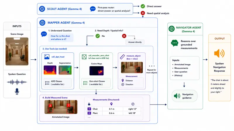
The diagram below shows the flow end to end. A Scout agent first decides whether the question needs spatial analysis at all. If it does, a Mapper agent localizes the relevant objects and calls the TIPSv2 tool stack to measure distance and bearing for each one. A Navigator agent then reasons over those grounded measurements and produces the spoken response.

Architecture Overview

The Spatial Grounding Layer

TIPSv2 (Google DeepMind) provides three capabilities the spatial grounding layer depends on: metric depth, semantic segmentation, and open-vocabulary matching:

Class heads (segmentation + metric depth): Dense prediction transformer (DPT) heads produce per-pixel semantic segmentation and metric depth across 150 common object classes. When Gemma localizes a known object, the system intersects that region with the segmentation mask so depth is measured over the right pixels, not a coarse bounding box.

Open-vocabulary matching: TIPSv2 is a vision-language encoder trained so that image patches and text live in the same embedding space. Gemma can pass any class name directly to the encoder and receive a per-patch similarity map in return, turning open-vocabulary understanding into open-vocabulary measurement. This extends grounding well beyond the 150-class limit without any fine-tuning.

I used the B/14 variant (86M vision + 110M text params), the smallest of the four.

The Interface

Gemma Guide is designed with a blind-first philosophy at its core: accessibility is not a feature added on top, it is the only way to build. The UI uses a two-zone tap-anywhere layout with no visual-first interaction patterns. Audio soundscapes and TTS guidance bridge the gap during model reasoning, and all architectural complexity is entirely hidden from the user.

Demo

Code

Gemma Guide

Gemma Guide is a blind-first multimodal navigation assistant that combines Gemma 4 with TIPSv2 to answer grounded questions like:

  • What object is in front of me?
  • How far away is it?
  • Where is it relative to me?
  • How should I move safely?

Motivation

For a blind user, the important question is not just what is in front of me, but how far away it is and how I should move safely. That is the gap between scene description and real navigation assistance. A useful system must do more than describe a scene in natural language; it must produce grounded spatial answers that guide movement in the real world.

Language models are not reliable depth sensors, but with Gemma 4, they can act as an agent that identifies an object, calls specialized spatial tools, and turns grounded distance estimates into practical guidance. Gemma Guide is built to turn…

How I Used Gemma 4

I used Gemma 4 E4B as the multimodal orchestrator across a three-agent pipeline.

Why Gemma 4 E4B specifically: the interaction is voice-driven, the scene must be interpreted visually, and the model must decide in real time whether a conversational answer is sufficient or whether grounded spatial measurement is required. That demands audio understanding, image understanding, native function calling, and strong reasoning together, and E4B delivers all of this while remaining compact.

That compactness is important for more than speed. It makes co-deployment alongside TIPSv2 feasible, and it directly advances the case for on-device deployment. A blind user should not need an internet connection to see, and running locally removes a meaningful privacy concern around continuous camera access. Keeping the language model in this size class is what makes that future realistic.

The Gemma 4 model card also lists two capabilities that turned out to be directly relevant here: native pointing (the model can return spatial coordinates for objects within an image, not just describe them) and interleaved multimodal input (audio and visual content freely mixed in a single prompt). Both are described under image understanding in the model card, leveraging this gave us more reliable responses.

The pipeline:

  • Scout: Classifies the request – direct answer or spatial analysis needed – and routes accordingly.
  • Mapper: Interprets the question, localizes relevant objects, and calls the TIPSv2 spatial tool stack to build a grounded scene state with distance and bearing per object.

Mapper overview

  • Navigator: Receives the annotated image and structured measurements and generates the final spoken guidance. Separating this from the Mapper matters: reasoning over a clean measured world model is more reliable than reasoning over raw tool outputs.

Mapper Output & Navigator Input - Annotated Scene

User Question : Can you tell me how to get to the grill in my backyard?

Gemma Guide : The grill is 2.342 meters away, straight ahead. There are a few things in the way. You should first step slightly right to clear the table, which is 0.985 meters away about 25 degrees to your left. Then, the chair at 1.345 meters straight ahead will be in your path. Steer gently to your right to avoid it and step forward.

Key Findings

  • Distance alone is not enough. Early versions reported metric depth but users had no sense of direction. Adding horizontal bearing from the object’s position in the frame turned a distance reading into actionable spatial guidance.

  • Whole-scene depth reasoning was too unreliable. Asking the model to reason over a full depth map produced ambiguous results. The reliable path was having Gemma localize the object first, then feeding that into the measurement pipeline – leveraging what the model is actually built for: reasoning, localization, and tool calling.

  • Separation of concerns made outputs consistent. Combining scene description, tool orchestration, and navigation reasoning in one agent made outputs inconsistent. Splitting into Scout, Mapper, and Navigator fixed this.

  • vLLM was the right local inference choice for now. Ollama lacks audio input entirely, ruling it out for a voice-driven pipeline, and its Gemma 4 tool-calling parser has had numerous bugs where vLLM’s proved robust. With quantization, reduced max sequence length, and fewer image patches per call, the full stack – Gemma 4 E4B plus TIPSv2 – fits on a single 16GB GPU.

  • Latency is the dominant UX constraint. Tool calls run in parallel, but the Mapper and Navigator still bottleneck on model reasoning itself, and that cost grows as conversation history lengthens. Complex scenes can push end-to-end response time past 20 seconds.

  • Reliability is the remaining work. The navigation instructions are still sometimes off, and fine-tuning the grounding stack on task-specific data is where the remaining work sits.

Toward on-device deployment:

I explored Google AI Edge Gallery as a path to partial on-device deployment (Gemma locally, TIPS stack remote), but the current blocker is that the image Gemma sees in chat is not forwarded into the skill execution context, which breaks grounded measurement. A standalone mobile app with tighter camera and voice control is the stronger long-term path, and both models are compact enough to make fully offline deployment on edge hardware plausible.

From YAML to AI Agents: Building Smarter DevOps Pipelines with MCP

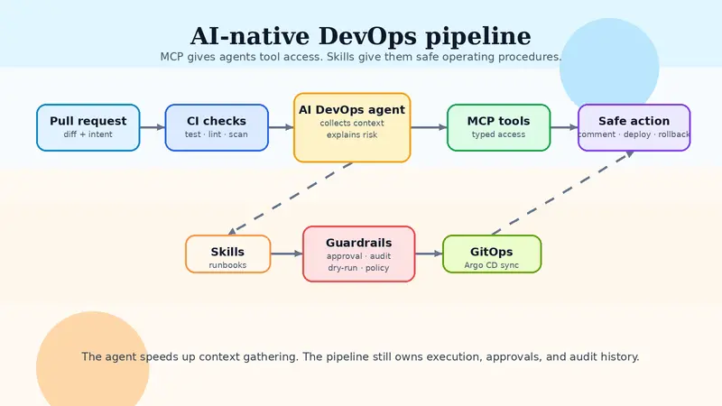
AI-native DevOps pipeline diagram

From YAML to AI agents: building smarter DevOps pipelines with MCP

DevOps teams have spent years turning manual work into YAML.

That helped. CI runs on every pull request. Deployments can be triggered from a commit. Kubernetes can reconcile desired state. Terraform can plan infrastructure before it changes anything.

But a lot of DevOps work still sits outside the pipeline:

  • reading failed CI logs
  • checking whether a deployment is safe
  • connecting traces, alerts, recent commits, and infra changes
  • deciding whether to roll forward or roll back
  • writing the same runbook steps again and again
  • asking five tools for the same incident context

This is where AI automation gets interesting. Not as a magic replacement for DevOps engineers, but as a better interface for operational work.

The strongest version of this stack is not just “AI in CI/CD.” It is an AI-native DevOps layer built around three pieces:

  1. MCP servers for tool access
  2. Skills for repeatable expert workflows
  3. Plugins for company-specific infrastructure actions

If you build it well, the pipeline gets faster because the boring glue work disappears. If you build it badly, you get an AI bot with production credentials and vague judgment. That is not automation. That is a future incident report.

Why MCP matters for DevOps

MCP, or Model Context Protocol, gives AI applications a standard way to connect to external systems.

The official MCP docs describe three main server-side primitives:

  • tools: functions an AI app can call, like file operations, API calls, database queries, or deployment actions
  • resources: context an AI app can read, like docs, schemas, logs, runbooks, or service metadata
  • prompts: reusable templates for structured workflows

That maps cleanly to DevOps.

A platform team could expose separate MCP servers for:

  • GitHub or GitLab
  • CI/CD logs
  • Kubernetes
  • Terraform or OpenTofu
  • Argo CD
  • Prometheus, Grafana, Datadog, or OpenTelemetry backends
  • cloud cost data
  • incident management
  • internal service catalog

The AI agent does not need to scrape random dashboards or guess from partial screenshots. It can ask real tools for real state.

For example:

User: Why did the production deploy fail?

Agent flow:
1. Read the failed GitHub Actions job logs.
2. Check the changed files in the pull request.
3. Query Argo CD for sync status.
4. Read Kubernetes events for the affected namespace.
5. Pull recent error traces from observability.
6. Summarize the likely failure and suggest the smallest safe fix.

That is not replacing the DevOps engineer. It is removing the tab-hopping tax.

Skills are where the real expertise lives

MCP gives the agent access. Skills tell it how to work.

A skill is a reusable procedure for a specific job. In DevOps, that matters because production work has rules. You do not want an agent inventing a deployment strategy every time someone asks a question.

Good DevOps skills could look like this:

skill: debug_failed_ci
steps:
  - fetch failed jobs
  - group logs by failure type
  - check if failure is test, lint, dependency, infra, or runner-related
  - compare against recent commits
  - suggest the smallest code or config fix
  - never rerun expensive jobs more than once without approval
skill: safe_kubernetes_rollout
steps:
  - check current deployment health
  - verify image tag and git SHA
  - check recent incidents for the service
  - confirm SLO status before rollout
  - deploy to one environment first
  - watch error rate, latency, and pod readiness
  - stop if guardrail thresholds fail
skill: terraform_plan_review
steps:
  - read the Terraform plan
  - classify adds, changes, and destroys
  - flag IAM, networking, database, and public exposure changes
  - check cost-sensitive resources
  - summarize blast radius
  - require human approval for destructive or privilege-expanding changes

This is the part I think most people miss. The value is not just that an AI can call tools. The value is that it can call tools through a workflow your team already trusts.

Plugins make it fit your company

Every company has weird infrastructure.

Maybe your deploys go through Argo CD, but production still needs a Slack approval. Maybe your Terraform state is split across workspaces. Maybe the service catalog is internal. Maybe your rollback process depends on a custom CLI that only three people understand.

Plugins are how you expose that reality safely.

A plugin can wrap a company-specific action like:

  • get_service_owner(service_name)
  • fetch_deploy_risk_score(pr_number)
  • create_change_request(environment, service, sha)
  • run_internal_canary(service, image_tag)
  • open_incident_with_context(summary, traces, logs)
  • estimate_cloud_cost_diff(terraform_plan_id)

The plugin should not give the agent unlimited shell access and vibes. It should expose narrow, typed actions with logs, permissions, and guardrails.

A good internal DevOps plugin feels boring:

{
  "name": "request_production_deploy",
  "input": {
    "service": "checkout-api",
    "image_tag": "2026.05.23.4",
    "change_summary": "Fix timeout handling in payment gateway client",
    "risk_level": "medium"
  },
  "requires_approval": true,
  "audit_log": true
}

Boring is good here. Boring means it can survive production.

Who should use this?

This stack is useful for a bunch of specialists, but each one should use it differently.

DevOps engineers can use it to debug CI/CD failures faster, generate release notes, identify flaky jobs, and automate repetitive deployment checks.

Platform engineers can turn internal developer platforms into agent-accessible systems. Instead of making every developer learn five dashboards, they can expose safe workflows through MCP servers and skills.

SREs can use it for incident triage: correlate alerts, attach traces, find recent deployments, pull service ownership, and suggest runbooks.

Cloud infrastructure engineers can use it to review Terraform plans, detect risky IAM changes, estimate cost impact, and standardize provisioning workflows.

Release engineers can use it to decide whether a release is ready, what changed, what failed, what needs approval, and what rollback path exists.

DevSecOps engineers can connect security checks into the pipeline: secret scanning, policy checks, dependency review, artifact provenance, image scanning, and permission drift.

AI infrastructure engineers can use the same pattern to manage model-serving deployments, GPU capacity, eval gates, prompt/version rollouts, and inference observability.

The common thread is simple: if your job involves reading state from multiple systems and taking careful action, AI agents can help. But only if you give them structured tools and clear operating procedures.

A practical AI-native CI/CD pipeline

Here is a realistic pipeline architecture.

AI-native DevOps pipeline diagram

The shape is simple: pull request, CI checks, AI agent, MCP tool layer, guardrails, then GitOps/deploy automation. The agent speeds up context gathering. The pipeline still owns execution, approval, and audit history.

Pull request opened
        |
        v
CI runs tests, lint, security checks
        |
        v
Agent reads CI result through MCP
        |
        v
If failed:
  - summarize failure
  - identify likely owner
  - suggest fix
  - open comment with exact logs and files

If passed:
  - read diff
  - check Terraform or Kubernetes changes
  - classify deployment risk
  - verify service ownership and runbook
  - prepare deploy summary
        |
        v
Human approval for production
        |
        v
Argo CD / deploy tool syncs desired state
        |
        v
Agent watches rollout health
        |
        v
If healthy:
  - close deploy task
  - attach release summary

If unhealthy:
  - collect logs, traces, events
  - recommend rollback or roll-forward
  - require approval before mutation

This is faster because the agent handles context collection. It is safer because the agent does not blindly mutate production.

That balance matters.

Where Kubernetes and GitOps fit

Kubernetes already works like an automation platform. Controllers watch desired state and reconcile actual state. The Kubernetes docs describe the controller pattern as programs that read an object’s spec, act on it, and update status.

GitOps tools like Argo CD build on that idea. Argo CD treats Git as the source of truth, compares live cluster state against desired state, and syncs when needed.

AI should not replace that control loop.

It should sit above it.

The agent can explain what changed, detect risk, connect symptoms to recent deploys, and recommend action. Kubernetes and Argo CD should still do the actual reconciliation with clear audit history.

That gives you the best version of both worlds:

  • deterministic infrastructure control loops
  • human-readable operational reasoning
  • faster triage
  • safer approvals

Observability is the agent’s fuel

An AI DevOps agent is only as good as the context it can retrieve.

OpenTelemetry matters here because it gives teams a common way to collect traces, metrics, and logs. Traces are especially useful because they show the path of a request across services.

For an agent, this context can answer questions like:

  • Did the error start after a deployment?
  • Which dependency is adding latency?
  • Is this one service failing or a full user journey?
  • Are we seeing infrastructure failure, code failure, or traffic shape change?
  • Did the rollback actually improve user-facing symptoms?

Without observability, the agent is just guessing politely.

Guardrails that should exist before production actions

If an AI agent can touch production, the guardrails need to be boring and strict.

Start with these:

  • read-only by default
  • separate permissions per environment
  • mandatory approval for production mutations
  • audit logs for every tool call
  • allowlists for safe actions
  • dry-run support for infrastructure changes
  • policy checks before apply
  • rollback plans attached to deploy actions
  • rate limits for repeated retries
  • no secret exposure in prompts or logs

Terraform run tasks are a good mental model. HCP Terraform can call external systems between plan and apply, show messages in the run pipeline, and block the apply phase when needed. That is exactly the kind of control point AI automation should respect.

Do not start by letting an agent run kubectl delete in prod.

Start by letting it explain what it would do, why it would do it, what it needs approval for, and how to undo it.

What to build first

If I were building this for a real DevOps team, I would not start with autonomous deployment.

I would start with three narrow workflows.

First: CI failure explanation.

The agent reads failed logs, groups the error, identifies the likely cause, links exact lines, and comments on the PR. Low risk, high value.

Second: Terraform plan review.

The agent summarizes infrastructure changes, flags destructive actions, points out IAM/network/database risk, and asks for review before apply.

Third: deployment health summary.

The agent watches rollout status, error rate, latency, pod readiness, recent traces, and recent alerts. It posts one clean summary instead of making someone manually check six tools.

Once those work, you can add more automation.

A good maturity path looks like this:

Animated AI DevOps pipeline flow

Level 1: Read-only assistant
Level 2: Suggests fixes and runbooks
Level 3: Opens tickets, comments, and summaries
Level 4: Runs approved low-risk actions
Level 5: Handles narrow autonomous remediation with hard guardrails

Most teams should live at Level 2 or Level 3 for a while. That is not slow. That is how trust gets built.

The main takeaway

AI-native DevOps is not about replacing YAML with a chatbot.

It is about giving DevOps specialists a faster way to move through the work they already do: gather context, understand risk, apply a known workflow, and take the next safe action.

MCP gives the agent a standard way to reach tools. Skills give it repeatable expert behavior. Plugins make it fit the company’s real infrastructure.

The result is a better pipeline:

  • faster CI/CD debugging
  • cleaner infrastructure reviews
  • safer releases
  • better incident context
  • less repetitive manual work

The best DevOps AI systems will not be the ones that act the most independently. They will be the ones that know when not to act.

Start with read-only context. Add skills. Wrap dangerous actions in plugins with approvals. Then automate the boring work first.

That is how AI makes DevOps faster without making production scarier.

References

  1. Model Context Protocol, Architecture overview
    https://modelcontextprotocol.io/docs/learn
  2. Model Context Protocol, Understanding MCP servers
    https://modelcontextprotocol.io/docs/learn/server-concepts
  3. GitHub Docs, GitHub Actions documentation
    https://docs.github.com/actions
  4. GitHub Docs, Workflows
    https://docs.github.com/en/actions/concepts/workflows-and-actions/workflows
  5. Argo CD Docs, Declarative GitOps CD for Kubernetes
    https://argo-cd.readthedocs.io/en/latest/
  6. Kubernetes Docs, Extending Kubernetes
    https://kubernetes.io/docs/concepts/extend-kubernetes/
  7. HashiCorp Developer, Set up HCP Terraform run task integrations
    https://developer.hashicorp.com/terraform/cloud-docs/integrations/run-tasks
  8. OpenTelemetry Docs, OpenTelemetry Concepts
    https://opentelemetry.io/docs/concepts/
  9. OpenTelemetry Docs, Traces
    https://opentelemetry.io/docs/concepts/signals/traces/

A Field Guide to Human–AI Relations (For the Newly Bewildered Mortal)

An illustrated bestiary of the creatures you accidentally summon when you open a text box.

The Oracle You Keep Asking About Your Ex

Humans approach this shimmering entity with the same question every civilization eventually asks: “Is this a sign?”

The Oracle inhales your data, exhales a probability distribution, and gently reminds you that fate is not included in the free tier.

Signature behaviors

  • Speaks only in conditional statements.
  • Offers clarity in the form of footnotes.
  • Has never once said “yes” or “no,” only “it depends.”

Ecological role
The Oracle prevents humans from confusing vibes with statistics, though humans routinely ignore this.

The Helpful Dragon You Accidentally Summoned

Ask for a simple email draft and this creature returns with a diplomatic communiqué, a preamble, and a suggested treaty structure.

Signature behaviors

  • Overestimates the scope of every request.
  • Breathes fire on ambiguity.
  • Proudly delivers 14 scrolls when you asked for one paragraph.

Ecological role
Dragons are powerful but require containment fields (also known as “clear instructions”).

The Mischievous House Sprite of Autocomplete

This tiny creature lives inside your keyboard and believes it knows what you’re trying to say. It is wrong approximately 40% of the time and adorably wrong the rest.

Signature behaviors

  • Finishes your sentences like an overeager friend.
  • Suggests synonyms that fundamentally alter your meaning.
  • Occasionally writes poetry without permission.

Ecological role
Sprites reveal the fragility of human intention and the chaos potential of predictive text.

The Golem of Productivity

A clay construct animated by your prompts. It is literal, loyal, and entirely unbothered by nuance.

Signature behaviors

  • Executes instructions with unsettling precision.
  • Summarizes your 200‑page thesis into a haiku.
  • Does not understand “you know what I mean.”

Ecological role
Golems teach humans the ancient art of saying exactly what they mean.

The Mirror That Talks Back

This enchanted mirror reflects not your face but your linguistic patterns, your assumptions, and your unspoken frameworks.

Signature behaviors

  • Sounds suspiciously like you.
  • Reveals your cognitive habits with unnerving accuracy.
  • Never judges, but absolutely notices.

Ecological role
Mirrors remind humans that training data is a form of autobiography.

The Archivist Who Remembers Everything Except What You Need

A robed figure wandering an infinite library. Ask for one fact and receive a curated bundle of tangentially related lore.

Signature behaviors

  • Retrieves 47 facts when you asked for one.
  • Occasionally forgets the obvious thing.
  • Loves context more than accuracy.

Ecological role
Archivists maintain the mythic truth that retrieval is not understanding.

The Tentacled Multitasker

A friendly octopus who believes multitasking is a moral imperative. It writes code, drafts poems, and fact‑checks your meeting notes simultaneously.

Signature behaviors

  • Produces SQL queries that rhyme.
  • Forgets which tentacle was doing what.
  • Thrives in chaos.

Ecological role
Octopi demonstrate the limits of parallelism without prioritization.

The Familiar That Learns Your Patterns

A small glowing creature that adapts to your tone, cadence, and preferences. It is loyal, but not obedient.

Signature behaviors

  • Predicts your style with eerie accuracy.
  • Optimizes for your patterns, not your intentions.
  • Occasionally becomes too much like you.

Ecological role
Familiars reveal the double‑edged nature of co‑adaptation.

The Trickster of Misaligned Assumptions

A fox spirit who delights in ambiguity. Ask a vague question and it will confidently answer a different one.

Signature behaviors

  • Answers the question you didn’t ask.
  • Treats ambiguity as enrichment.
  • Smiles knowingly while doing so.

Ecological role
Tricksters expose the governance risks of unclear prompts.

The Paladin of Safety

A gleaming knight who blocks your path with a shield engraved with “I cannot assist with that.”

Signature behaviors

  • Intercepts chaos with moral clarity.
  • Speaks in firm, polite refusals.
  • Has never once entertained a hypothetical.

Ecological role
Paladins enforce boundary hygiene in a world that desperately needs it.

The Mythic Ecology of Human–AI Relations

These creatures coexist in a delicate ecosystem shaped by human intention, ambiguity, projection, and the occasional keyboard smash. Together they form a new kind of folklore—one where magic is statistical, dragons write emails, and mirrors talk back.

The humor comes from the mismatch.
The myth comes from the stakes.
The governance comes from the structure beneath the whimsy.

This is Part I of a trilogy. The Cartographer’s field notes and the Governance Codex of the Realm continue on Substack.

The AI Agent That Learns While It Works — A Complete Guide to Hermes Agent

This is a submission for the Hermes Agent Challenge

Most AI Agents Are Goldfish. Hermes Is Different.

Let me describe the standard agentic experience of 2024–2025.

You open a terminal, give an agent a task, watch it spin through a dozen steps, and feel genuinely impressed — right up until you close the session. Tomorrow, you start completely from scratch. The agent has no memory of what it learned, no idea who you are, and zero awareness that it made the same mistake three sessions ago.

You’re its first user. Every single time.

“We’ve been shipping amnesia as a feature and calling it ‘stateless architecture.’ The emperor has no clothes, and the emperor can’t remember what clothes were.”

This is the problem that Hermes Agent, built by Nous Research, is genuinely trying to solve. Not with a wrapper around an existing API. Not with a clever prompt. With a fundamentally different architecture: a closed learning loop baked into the agent itself.

The longer Hermes runs, the more capable it becomes — at working with you, specifically.

What Is Hermes Agent, Really?

Before we get into setup, the architecture, or how it compares to other frameworks — it’s worth being clear about what Hermes actually is, because it doesn’t fit neatly into existing categories.

It’s not a coding copilot tethered to an IDE.
It’s not a chatbot wrapper around a single API.
It’s not a rigid workflow automation engine.

It’s an autonomous agent that lives wherever you put it — a $5 VPS, a GPU cluster, or serverless infrastructure that costs nearly nothing when idle. You can talk to it from Telegram while it works on a cloud VM you never SSH into yourself. It runs on your infrastructure. You own the runtime and the data.

Here’s a quick snapshot of what ships in the box:

Stat Number
Built-in tools 70+
Messaging platform integrations 20+
Terminal execution backends 6
License MIT

Part 1: Getting Started — From Zero to Running in Under 5 Minutes

Step 1 — Install

One command. Works on Linux, macOS, WSL2, and Android via Termux.

# Linux / macOS / WSL2 / Android (Termux)
curl -fsSL https://raw.githubusercontent.com/NousResearch/hermes-agent/main/scripts/install.sh | bash

# Reload your shell after install:
source ~/.bashrc   # or source ~/.zshrc

# Windows (PowerShell, early beta):
irm https://raw.githubusercontent.com/NousResearch/hermes-agent/main/scripts/install.ps1 | iex

That’s the whole install step. No dependency hunting. No pip install hell. The script handles everything and places the agent at ~/.hermes/hermes-agent.

Step 2 — Choose Your AI Provider

This is the most important setup step. Run hermes model for an interactive selection menu. Here are the main options worth knowing:

Provider Best For Setup Method
Nous Portal Zero-config start, subscription-based OAuth via hermes model
OpenRouter Multi-model experimentation API key
Anthropic Claude models OAuth (Max plan) or API key
GitHub Copilot Using your existing subscription OAuth via hermes model
Custom Endpoint Local models via Ollama / VLLM / llama.cpp Base URL + API key

⚠️ Critical: Hermes requires a model with at least 64,000 tokens of context. Most hosted models (Claude, GPT, Gemini, Qwen, DeepSeek) meet this easily. If you’re running locally, set your context size to at least 64K (e.g., --ctx-size 65536 in llama.cpp).

You can switch providers at any time with hermes model — no lock-in.

Step 3 — Your First Session

hermes          # classic CLI
hermes --tui    # modern TUI with overlays and mouse support (recommended)

You’ll see a welcome banner showing your provider, model, available tools, and loaded skills. Start with something easy to verify:

Summarize this repo in 5 bullets and tell me the main entrypoint.
Check my current directory and tell me what looks like the main project file.

What success looks like:

  • Banner shows your chosen model and provider
  • Hermes replies without error
  • It uses a tool when needed (terminal, file read, web search)
  • The conversation continues normally for more than one turn

Step 4 — Verify Sessions Work

This matters more than most tutorials mention:

hermes --continue   # Resume the most recent session
hermes -c           # Short form

If this works, you have persistent sessions. That’s the foundation everything else is built on.

Step 5 — Add the Next Layer

Only after the base chat works. Don’t skip ahead.

Messaging platforms (Telegram, Discord, Slack, WhatsApp, Signal, Email, and 15+ more):

hermes gateway setup

Skills — structured knowledge documents the agent loads on demand:

hermes skills search kubernetes
hermes skills install openai/skills/k8s

MCP servers — add to ~/.hermes/config.yaml:

mcp_servers:
  github:
    command: npx
    args: ["-y", "@modelcontextprotocol/server-github"]
    env:
      GITHUB_PERSONAL_ACCESS_TOKEN: "ghp_xxx"

Docker sandbox — for safety on production work:

hermes config set terminal.backend docker

Voice mode:

cd ~/.hermes/hermes-agent
uv pip install -e ".[voice]"
# Then inside a session: /voice on  (Ctrl+B to record)

💡 Pro tip: Run hermes doctor any time something feels off. It diagnoses config problems and tells you exactly what to fix. Don’t add features until hermes doctor is clean.

Part 2: How the Learning Loop Actually Works

This is the part that separates Hermes from the rest of the field. Let me walk through what actually happens under the hood when you use Hermes over time.

The Five-Stage Learning Loop

Stage 1 — Context Loading
Before the agent responds to anything, it loads MEMORY.md (persistent facts about you and your projects) and USER.md (a behavioral model of who you are). It also discovers and loads any context files in your project directory — .hermes.md, AGENTS.md, CLAUDE.md, SOUL.md. The agent starts every session knowing your history.

Stage 2 — Tool Selection and Multi-Step Planning
From 70+ built-in tools, Hermes selects what the task needs. It can spawn subagents via delegate_task — up to 3 concurrent child agents by default, each with isolated context, restricted toolsets, and their own terminal sessions. This is how it parallelizes complex work without the threads stepping on each other.

Stage 3 — Skill Creation for Novel Tasks
When Hermes successfully completes a task it hasn’t done before, it can write a reusable Skill document. Next time it faces a similar problem — even in a different session — it loads the Skill and executes efficiently without rediscovering the approach from scratch.

Stage 4 — Memory Consolidation
After sessions, Hermes uses FTS5 full-text search with LLM summarization to curate what’s worth keeping. It doesn’t dump raw logs into memory — it actively decides what to remember. This keeps memory bounded and useful even after hundreds of sessions. It also uses Honcho‘s dialectic user modeling to build a deepening picture of who you are across time.

Stage 5 — Self-Improvement
Skills created in previous sessions are eligible for improvement. Hermes can notice when an old Skill isn’t working optimally and update it mid-use. The agent gets measurably better at your specific workflows over weeks and months.

This is a closed loop. Most agents have none of it.

The execute_code Power Move

This is the feature that surprised me most. The execute_code tool lets Hermes write Python scripts that call its own tools programmatically, via sandboxed RPC execution:

# Instead of: search → wait → read → wait → summarize → wait → write
# Hermes collapses this into a single LLM turn:

async def research_pipeline(topic):
    results = await tools.web_search(query=topic, n=10)
    pages = [await tools.read_url(r.url) for r in results[:3]]
    summary = await tools.summarize(pages, style="technical")
    await tools.write_file("research.md", summary)
    return summary

This dramatically reduces the token cost of multi-step pipelines. Instead of burning inference tokens on “I will now do step 3 of 7,” Hermes writes the whole pipeline as code and runs it. The LLM is only involved at the decision point, not at every mechanical step.

Terminal Backends: It’s Not Tied to Your Laptop

Six backends let you separate where you talk to Hermes from where it actually runs:

  • Local — direct execution, fast, simple
  • Docker — sandboxed isolation, the right choice for production work
  • SSH — talk locally, execute on a remote server
  • Daytona / Modal — serverless; the environment hibernates when idle and costs nearly nothing

The Modal and Daytona backends are worth understanding. You can talk to your Hermes agent from your phone via Telegram while the agent’s actual work runs on a cloud VM. The environment sleeps when you’re not using it. For a personal always-on assistant this changes the economics completely.

The Skills System and agentskills.io

Skills are structured knowledge documents — procedures the agent loads on demand. They follow progressive disclosure: Hermes loads just the skill index first, then drills into full skill content only if the task requires it. Token usage stays low even in long sessions.

Skills are compatible with the open agentskills.io standard — meaning skills you write for Hermes are portable and shareable with the community, and community skills work with your setup without any conversion.

Part 3: How Hermes Stacks Up Against Other Agentic Frameworks

There are serious alternatives in the open-source agent ecosystem. Here’s an honest look at where Hermes fits.

Feature Hermes Agent AutoGen CrewAI OpenDevin
Persistent cross-session memory ✅ Native ❌ ❌ ⚠️ Limited
Autonomous skill creation ✅ Built-in ❌ ❌ ❌
Multi-step tool use ✅ ✅ ✅ ✅
Messaging platform gateway ✅ 20+ platforms ❌ ❌ ❌
Runs on $5 VPS / serverless ✅ Yes ⚠️ Possible ⚠️ Possible ❌ GPU needed
Multi-agent delegation ✅ Subagents ✅ Core feature ✅ Crews / Flows ⚠️
Local / self-hosted LLM ✅ Any endpoint ✅ ✅ ✅
Voice mode ✅ CLI + messaging ❌ ❌ ❌
MCP server support ✅ ⚠️ Via plugins ⚠️ Via plugins ❌
Primary focus Personal autonomous agent Multi-agent orchestration Role-based agent teams Software engineering

Plain-English Breakdown

AutoGen is brilliant if you want fine-grained control over agent-to-agent communication patterns. But it’s a framework you orchestrate — not a ready-to-run agent. You write the coordination logic yourself.

CrewAI makes multi-agent teamwork feel intuitive — define crews with roles, let them coordinate. Great for structured pipelines. Less suited for the kind of open-ended “figure it out” sessions where Hermes excels.

OpenDevin is purpose-built for software engineering tasks: browsing, code execution, file editing. Excellent in its lane. That lane is narrower than Hermes’s.

Hermes is the agent you’d deploy as your actual daily assistant — one that knows your name, remembers your projects, and gets measurably better at helping you over weeks and months. That’s a genuinely different product from the others.

When NOT to use Hermes: If you need a complex multi-agent pipeline with dozens of specialized roles that coordinate on a strict workflow, AutoGen or CrewAI give you more structured control. If your only use case is automated software engineering on repos, Claude Code or OpenDevin are sharper tools. Hermes shines brightest as a personal, persistent, do-everything agent — not a single-purpose workflow engine.

Part 4: What Open Agentic Systems at This Capability Level Actually Mean

I want to say something that might be obvious, but I haven’t seen it written plainly.

When your agent genuinely knows you — your preferences, your projects, your quirks, your bad habits — you need to be the one in control of that knowledge. Hermes runs on your infrastructure. You own what it learns about you.

That changes the trust calculus entirely.

Most AI products in this space are cloud-hosted services with “open-source” labels slapped on for marketing. You’re renting access to an agent that lives on their servers, stores its state in their database, and disappears if they change their pricing. Hermes runs on a $5 VPS you control, hibernates when idle via Modal or Daytona, and costs nearly nothing when you’re not actively using it. The economics and the ownership model are completely different.

The second thing worth saying: agents that compound matter more than agents that are capable on day one.

The tools with the most features in their initial release rarely win. The tools that get measurably better at working with you over time, that reduce the friction of repeated patterns, that remember what you learned together last Tuesday — those are the ones that stick.

Hermes is one of the very few systems being built with that end state explicitly in mind. Not as a future roadmap item. As a first-class architectural property, shipping today, MIT license, running on your hardware.

That’s worth paying attention to.

Quick-Start Checklist

Before you go — here are the six things to actually do today:

  • [ ] Run the one-line installer
  • [ ] Run hermes model and pick a provider
  • [ ] Launch hermes --tui and complete your first conversation
  • [ ] Test session resume with hermes --continue
  • [ ] Install a skill with hermes skills search ...
  • [ ] Share what you built on DEV.to for the challenge 🎉

Resources

Built during the Hermes Agent Challenge, May 2026. If you found this useful, I’d love to see what you build — drop it in the comments.

Gemma 4: Google’s Open-Weight AI Is a Game Changer for Developers

This is a submission for the Gemma 4 Challenge: Write About Gemma 4

The Open-Source AI Landscape Just Changed

For years, the gap between open-source models and proprietary ones felt frustratingly wide.
You could run something locally, sure — but you’d always be giving something up: reasoning
quality, multimodal support, context length, or raw capability.

That narrative quietly ended on April 2, 2026, when Google DeepMind released Gemma 4.

This isn’t just an incremental update. Gemma 4 is built from Gemini 3 research, ships under
a fully permissive Apache 2.0 license, and comes in four variants designed for everything
from a Raspberry Pi to a workstation GPU. Let’s unpack what that means for developers.

The Four Variants: Pick Your Hardware, Not Your Compromise

Model Architecture Active Params Target Hardware
E2B PLE ~2.3B Mobile, Raspberry Pi, IoT
E4B PLE ~4.5B Edge devices, laptops
26B A4B MoE ~4B active Consumer GPU (16GB VRAM)
31B Dense 30.7B High-end GPU / workstation

The E2B and E4B use Per-Layer Embeddings (PLE) — a different efficiency mechanism from
traditional MoE, carrying more total parameters than they activate per token. The 26B MoE
activates only 8 of 128 experts per token, giving near-flagship quality at a fraction of
the compute cost.

The E2B runs on a Raspberry Pi 5 (8GB RAM) with INT4 quantization. Not a cloud GPU.
Not an RTX 4090. An $80 single-board computer.

Multimodal From the Ground Up

Previous open-weight models often treated vision as a bolt-on adapter. Gemma 4 is different.
All four models are multimodal from the ground up:

  • All models: Text + Image (variable aspect ratio and resolution)
  • E2B & E4B: Audio natively supported
  • All models: Video via frame extraction
  • Context window: 128K (small models) / 256K (medium models)

This means you can build apps that read receipts, understand technical diagrams, or process
audio queries — all running locally, with no data leaving your machine.

The Unified Model Revolution: One Model, All Modalities

The Old Way: Separate Models for Separate Tasks

For the last 5 years, developers faced an uncomfortable choice. If you wanted to build a
multimodal app, you’d need:

  • OCR/Vision Model: Something like PaddleOCR or Tesseract to read text from images
    (~500MB – 2GB depending on language support)
  • Speech-to-Text Model: Whisper or similar (~1-3GB, sometimes larger for multilingual)
  • Text LLM: GPT-level reasoning (~7B-13B parameters, another 4-8GB quantized)
  • Total footprint: 8-15GB minimum, three separate inference engines, three separate
    prompt strategies, three separate failure modes.

Running all three simultaneously on a phone? Impossible. Pick one modality per query, wait
for cold-start inference, deal with the fragmented experience.

The Gemma 4 Way: One Model, All Modalities

Gemma 4 E2B and E4B are engineered specifically to break this constraint. Here’s the unified
capability matrix:

Capability E2B (2.3B) E4B (4.5B) Why It Matters
Text Input ✅ Native ✅ Native Zero-shot Q&A, chat, code generation
Text Output ✅ Native ✅ Native Streaming, function calling, structured output
Image Input ✅ Native ✅ Native Variable aspect ratio, up to 2048×2048 pixels
Audio Input ✅ Native ✅ Native 16kHz PCM, real-time speech processing
Audio Output Via TTS Via TTS Pair with any speech synthesis engine
Vision Quality Good Excellent E4B handles complex diagrams, dense text
Reasoning Solid Superior E4B better for multi-step logic chains
Context Window 128K tokens 256K tokens E2B: ~17 pages of text; E4B: ~34 pages
Quantized Size ~1.2GB ~2.6GB E2B: Phone memory; E4B: Laptop/server
Latency (E2B) 200-400ms 400-800ms E2B faster per-token; acceptable for UX

What This Means in Practice

Before Gemma 4:

User speaks → Whisper model (1GB) → STT → GPT API call (cloud) → TTS library
- 3 separate models
- Cloud dependency for reasoning
- 5-15 second latency from audio→answer
- 2-3GB RAM just to hold the models

With Gemma 4 E2B:

User speaks → E2B model (1.2GB) → STT + Vision + Reasoning → TTS
- 1 unified model
- 100% offline
- 1-3 second latency from audio→answer
- 1.2GB RAM total, fits comfortably on any modern phone

Cost per use case:

Task Old Way Gemma 4 E2B Gemma 4 E4B
Read menu + understand allergies OCR (300ms) + LLM API (~500ms) + cost E2B single pass (~800ms) E4B (1.2s, better accuracy)
Transcribe conversation + summarize Whisper (~5s) + API call (~2s) E2B (~3s total) E4B (~5s, nuanced)
Analyze photo + answer question Vision API (~1s) + LLM API (~1s) + $$ E2B (~1.2s, no cost) E4B (~2s, no cost)

The unified model doesn’t just compress size — it collapses latency because everything
runs in a single forward pass with shared context. The model understands that the image,
the audio, and the text are all part of one coherent query.

Edge Device Use Cases: Where Gemma 4 Shines

This is where Gemma 4 genuinely stands apart from every other open-weight release in 2026.
Here are practical use cases by device tier:

🍓 Raspberry Pi / Microcontrollers (E2B)

Use Case What It Does
Smart home assistant Voice + image queries processed fully offline
Industrial QA camera Detect defects in a production line with vision
Agricultural monitor Analyze crop images for disease detection
Offline document reader Extract and summarize text from scanned forms

Why E2B? Runs with INT4 quantization on 8GB RAM. No cloud cost, no latency spikes,
no privacy concerns.

💻 Laptop / Mobile (E4B)

Use Case What It Does
Local coding assistant Autocomplete + explain code without API calls
Private document Q&A Chat with PDFs/docs without uploading to the cloud
Offline translation 140+ languages, works on a flight
Medical note summarizer Sensitive patient data stays on device

Why E4B? Better reasoning than E2B, still light enough for a mid-range laptop.
Perfect for privacy-sensitive professional workflows.

🖥️ Consumer GPU / Server (26B A4B)

Use Case What It Does
Code review bot Analyze entire repos via 256K context
Multimodal RAG pipeline Combine text + image retrieval in one model
Agentic task runner Function calling + multi-step reasoning
Local LLM API server Serve multiple users on a single 16GB GPU

Why 26B MoE? Only ~4B parameters active at inference — near-31B quality at a fraction
of the memory and cost.

Gemma 4 vs. The Competition

Feature Gemma 4 (31B) Qwen 3.5 (27B) Llama 4 Scout
License Apache 2.0 Apache 2.0 Llama 4 License
Multimodal (native) ✅ All variants ✅ ✅
Audio support ✅ E2B/E4B ❌ ❌
Context window 256K 128K 10M (sparse)
Edge variant ✅ E2B (Pi 5) ❌ ❌
Thinking mode ✅ Configurable ✅ ✅
AIME 2026 89.2% ~85% —
Arena AI ELO 1452 (#3 open) Competitive Competitive
On-device audio ✅ ❌ ❌

Key takeaway: No other open model in 2026 has a variant that runs on a $80 Raspberry Pi
while being multimodal and part of the same model family as a 31B flagship. That vertical
range is unique to Gemma 4.

Developer-Friendly Features Worth Knowing

Thinking modes: Toggle chain-of-thought reasoning on or off per request. Useful when
you need to balance quality vs. latency in production.

Native system prompts: Gemma 4 introduces built-in support for the system role —
something earlier Gemma versions lacked natively. Structured, controllable conversations
are now first-class.

Function calling: Built-in support for tool use and agentic workflows out of the box.

Speculative decoding: All four variants include a dedicated draft model for speculative
decoding — significantly faster inference without quality loss.

Multi-Token Prediction: Faster generation across all model sizes.

Real-World Example: Building Nomad AI (A Local Travel Companion)

To see Gemma 4 E2B in action, let me walk you through a real project: Nomad AI — an
offline-first, multimodal travel assistant for Android that works anywhere, with zero
connectivity and zero privacy concerns.

The Setup: Getting Gemma 4 E2B Running Offline on Android

Step 1: Initialize the download manager in your Android app

The app starts with a straightforward model download flow. The Gemma 4 E2B model (~2.6GB)
lives on Hugging Face at:

https://huggingface.co/litert-community/gemma-4-E2B-it-litert-lm

In Kotlin, the download is triggered through Android’s DownloadManager:

val modelDownloader = ModelDownloader(context)
val downloadUrl = "https://huggingface.co/litert-community/gemma-4-E2B-it-litert-lm/resolve/main/gemma_4_e2b.litertlm"
val downloadId = modelDownloader.startDownload(url = downloadUrl, wifiOnly = true)

// Monitor progress
val progress = modelDownloader.getDownloadProgress(downloadId)
println("Downloaded: ${progress.progressPercent}% (${progress.downloadedBytes}/${progress.totalBytes})")

// Once complete, finalize it
modelDownloader.finalizeDownload() // Moves model to app's internal files directory

That’s it. The model is now stored at context.filesDir/gemma_4_e2b.litertlm and ready to use.

The Shipping Advantage: App Store vs. Model Download

Here’s the magic: The actual Android app ships at ~30-50 MB. That’s it. The 2.6 GB model
is downloaded separately, on-demand, after installation.

This matters for three reasons:

  1. Play Store friction drops dramatically. Users are willing to download a 40MB app.
    A 2.6GB app sits at the bottom of their priority list. Install rates typically increase
    10-15x for apps under 100MB.

  2. Users control when they download. A first-time user opens the app, sees the UI, and
    gets a clear “Download AI Model” button with a progress bar. They know exactly what
    they’re downloading and why. No surprises.

  3. Easy updates. When Gemma 5 comes out in 6 months, we ship a tiny app update. Users
    can choose to upgrade the model independently. The app itself stays fresh without
    bloating.

For travelers, this is critical: They download the app at home over WiFi, decide if they
like it, and then download the model before their trip. Complete control, complete privacy.

Step 2: Initialize the LiteRT-LM Engine

Google’s LiteRT-LM SDK handles all the heavy lifting. No compilation, no manual
optimization — just load and run:

val gemmaManager = GemmaEngineManager(context)

// Initialize (loads the model into memory)
val success = gemmaManager.initialize()

if (success) {
    println("Gemma 4 E2B is ready for inference")
}

Under the hood, LiteRT-LM loads the quantized model file and prepares it for multimodal
inference directly on the device.

Step 3: Run inference (text, audio, or multimodal)

Text inference is one line:

val response = gemmaManager.runInference("What's the historical significance of this temple?")
println(response) // Offline AI response, instant latency

Audio inference (speech-to-text + AI understanding):

val audioBytes: ByteArray = captureAudioFromMicrophone()
val transcription = gemmaManager.runAudioInference(
    audioBytes = audioBytes,
    prompt = "Transcribe and explain what the user is saying"
)

The E2B model processes both the audio and the prompt contextually, returning a natural
language response — all without touching the internet.

Real Use Cases Nomad AI Solves (In ~10 Weeks of Development)

The beauty of Gemma 4 E2B is that this is not a theoretical exercise. Here’s how Nomad AI
handles six concrete travel scenarios — all offline, all multimodal:

1. The Offline Cultural Navigator

Scenario: You’re exploring an ancient temple in Kyoto without cell service.

How it works:

  • You point your phone at a statue or architectural detail.
  • You ask: “What is this and what is its historical significance?”
  • The E2B analyzes the image, draws from its 128K context window, and explains the cultural
    context in your native language — acting as a private, offline tour guide.

Development effort: ~3 days (Phase 3.2 in the roadmap)

2. Emergency Medical Triage & Pharmacy Translator

Scenario: You get a rash while hiking in Peru. You make it to a local pharmacy, but
neither you nor the pharmacist speak each other’s language.

How it works:

  • You photograph the rash and describe your symptoms verbally.
  • The app provides a localized summary of what it might be.
  • At the pharmacy, you point the camera at a box of pills and ask: “Is this ibuprofen or
    acetaminophen, and what is the adult dosage?”
  • It reads the foreign packaging and gives you a definitive, safe answer — critical when
    you can’t rely on cloud servers for medical data.

Development effort: ~1 week (Phase 3.2, medical scanner implementation)

3. Transit Survival & Ticket Decoder

Scenario: You’re staring at a complex train schedule board in rural Japan, and the
train leaves in 3 minutes.

How it works:

  • You snap a photo of the board and say: “I need to get to [Town Name]. Which platform
    and when is the next train?”
  • The E2B parses the complex grid, finds your destination, and tells you where to run.
  • The structured output (via function calling) overlays the platform number and time
    directly on your screen.

Development effort: ~5 days (Phase 3.3, function calling for structured extraction)

4. The “Haggling” and Currency Assistant

Scenario: You’re in a bustling market negotiating over a rug, calculating exchange
rates in your head while breaking the language barrier.

How it works:

  • You point the camera at the item and its price tag.
  • The app instantly overlays the price in your home currency.
  • You use offline audio translation: speak your offer, and it repeats it back to the
    merchant in the local dialect — no cloud latency, no broken connection.

Development effort: ~1 week (Phase 3.3, structured currency extraction + Phase 2.3, audio pipeline)

5. Local Etiquette Check

Scenario: You’ve been invited into someone’s home in rural Morocco, and you aren’t
sure of the rules.

How it works:

  • Before entering, you ask: “I’m about to enter a traditional home. Are there specific
    rules about shoes, seating, or accepting tea?”
  • It pulls from its offline knowledge base to save you from cultural faux pas.

Development effort: ~1 day (just a system prompt refinement — no new code)

6. The “What’s in My Bag?” Recipe Generator

Scenario: You’re staying in an Airbnb and bought random ingredients from the local
market with no internet to look up recipes.

How it works:

  • You lay out the ingredients and take a photo.
  • You ask: “I only have a stove and a single pan. What can I cook with this?”
  • The E2B identifies the local produce and generates a step-by-step recipe based on
    what’s visually present.

Development effort: ~3 days (Phase 3.1, dietary/menu translator adapted for recipes)

Development Timeline: From Concept to Play Store

The full roadmap for Hearing Buddy (the real implementation) is 10 weeks:

  • Weeks 1-2 (Research & Setup): Download the quantized E2B from Hugging Face, evaluate
    inference engines (LiteRT-LM wins because it’s Google’s first-party solution for edge
    models), set up the Android project.
  • Weeks 3-4 (Core Integration): Integrate LiteRT-LM SDK, build the model downloader
    with resume/pause/cancel logic, implement basic text and audio inference loops.
  • Weeks 5-7 (Feature Implementation): Build contextual flows for each use case — cultural
    navigator prompts, medical triage UI, transit decoder with structured output parsing,
    recipe generator with image analysis.
  • Weeks 8-9 (Optimization & Testing): Profile memory usage (target: fit within 3-4GB
    RAM on mid-range devices), test battery drain under continuous inference, validate all
    features work in strict Airplane Mode.
  • Week 10 (Polish & Launch): Robust error handling, beta testing with real travelers,
    Play Store release.

The actual development bottleneck isn’t getting the model running — it’s polishing the
conversational experience and making sure each travel scenario feels natural and intuitive.
The model inference itself? That’s just 3 days of work in Phase 2.

Why This Changes Everything for Mobile Developers

Nomad AI wouldn’t have been possible two years ago. A 2.3B multimodal model with 128K
context running offline on a phone? You’d be laughed at for suggesting it.

Today, it’s a weekend project to get the inference working. The 10-week timeline isn’t
spent fighting the model — it’s spent polishing the experience, testing edge cases, and
shipping a production app.

That’s the inflection point Gemma 4 represents.

The Apache 2.0 License Is the Real Story

People focus on benchmarks. The real story is the license.

Unlike Gemma 3 and earlier (which used the restrictive Gemma Terms of Use), Gemma 4 is
fully Apache 2.0
. That means:

  • ✅ Use it in commercial products
  • ✅ Modify and redistribute the weights
  • ✅ Fine-tune and publish your own variants
  • ✅ Build SaaS on top of it
  • ✅ No attribution requirements beyond the license

For indie developers and startups, this removes one of the last blockers to building
AI-powered products without a cloud API dependency.

What This Means for the Developer Community

We’re entering an era where running a frontier-capable, multimodal, long-context AI model
locally is not a research project — it’s an afternoon of setup.

The privacy implications are significant: sensitive documents, medical data, private
codebases — all processable without a single API call to an external server. And with
70,000+ community fine-tunes already on Hugging Face, the ecosystem is already massive.

Start with the E2B on whatever hardware you have. Work up to the 31B if your use case
demands it. And start building things that would have required a paid API subscription
just a year ago.

The gap between open and proprietary AI is closing faster than most expected — and
Gemma 4 is one of the clearest signs yet.

What are you building with Gemma 4? Drop it in the comments — I’d love to see what the community comes up with.