🧞‍♂️Transform unstructured PDFs Job Offers into a dataset w. gemma4:2b

This is a submission for the Gemma 4 Challenge: Build with Gemma 4

🤔 About the power of collections and our ability to compare things

First a bit of philosophy.

Did you notice how we tend to align things, tend to shape things so they can be aligned, compared (based on a common attributes like color, weight,…).

Comparing objects is much easier when they share common structure, then we can use attributes to get more knowledge, produce KPIs, make clever choices and put things in evidence.

👉 Well the same happens with machines : it’s much much easier to compare and manage documents when they share a same structure.

This is the very core idea that motivated this work to explore how Open Source AI could help in a very pragmatic way… and feel the opportunities it opens with concrete prototypes.

🙋 What I Built

I’ve built a whole real life and live data pipeline that takes as input Open Data Public Sector Job offers (dataset/avis-de-vacances-de-poste-avp-drhfpnc) :

  • csv
  • Raw PDFs

Then,

  1. From a dedicated GH repo adriens/avps I’ve prepared a whole structured mix of md thanks to csv
  2. Then from the GH Action I did transform brut raw PDFs with pypi.org/marker-pdf into markdown
  3. I ended to publish a dedicated Zensical gh-pages website : adriens.github.io/avps

Next, this is where things go really interesting : I wanted to be able to compare job offers the one against the others… but markdown were far too much different the one from others :

  • Not the same number of sections
  • Not the same section titles : hard skills, soft skills, missions,…
  • Not the same levels of sections
  • Not necessarly itemized the one
  • Not the same style at all (section levels, CAPITALs, email, cities…)

… which made it very hard… or even impossible to compare them amongs the others… or even crazier : put them in a traditional SQL structured database.

👉 This is where gemma4:2b comes in to create a very well and consistent set of markdowns that can then be used for various use cases :

  • Create very well structured ePub to read job offers on the go (and docx)
  • Create a very clean and well organized PDF : very easy to load in assistants, print or to drop in any assistant
  • Deliver structured data with clean json files
  • Make a duckdb database and perform SQL on the data by using the now well structured markdowns, which made it possible to open unprecedented and exciting reporting opportunities (here in duckdb)
  • Share all this as a dataset on Kaggle
SELECT '--- RÉPARTITION DES COMPÉTENCES PAR DOMAINE ---'
as titre_report;
SELECT domaine, count(*) as nb_competences 
FROM savoir_faire 
GROUP BY 1 ORDER BY 2 DESC;

// Detect dark theme
var iframe = document.getElementById(‘tweet-2055533578021396775-622’);
if (document.body.className.includes(‘dark-theme’)) {
iframe.src = “https://platform.twitter.com/embed/Tweet.html?id=2055533578021396775&theme=dark”
}

🎯 Problems it solves

In input we really had very various kind of PDF documents, and no structured tabular data, now, they both are delivered as :

  • Well formated and structured markdown
  • A real database that embeds data as tables and views for advanced SQL reporting and charting
  • Ready to use and perfectly well structred ePub and PDF documents, very easy for LLMs to understand

🤗 Experience it creates

The experience is rather an data experience as thanks to data normalisation and standardization we can load and compare job offers, which make job search and indexing much much more efficient, whatever the input.

Last but not least, using gemma4:2b-it proves that great things can be achieved even with small resources and that well prepared data opens so many intelligence opportunities, without having to deal with frontier models as “the output I got is good enough”.

🍿 Demo

💰 The benefits : then and now

Below the benchmark of markdown before and after

⚖️ Benchmark : marker-pdf vs. marker-pdf ➕ gemma4:e2b

Below some results:

Structure consistency:

📊 Analytics on top of database

One the well-structured json could be produced from the markdown I could efficiently load them into a duckdb database and do some reporting see AVPS DRHFPNC – Les pdf en SQL avec duckdb Kaggle notebook :

// Detect dark theme
var iframe = document.getElementById(‘tweet-2055751934301380738-928’);
if (document.body.className.includes(‘dark-theme’)) {
iframe.src = “https://platform.twitter.com/embed/Tweet.html?id=2055751934301380738&theme=dark”
}

📜 Code

🎁 Goodies

💡 How I Used Gemma 4

I chose google/gemma-4/transformers/gemma-4-e2b-it from kagglehub as I had a huge amounf of data to load (all New-Caledonia ones) and a restricted amount of time on Kaggle as well as small GPUs.

Also my intent was to be able to run this code one day onPrem on my very own hardware so I decided to stay as little as possible.

🤔 What remains to do…

Try to:

  • Add an evaluation phasis to check output consistency
  • Try to switch to CPU mode so the Notebook can be scheduled without exceeding the maximum Kaggle window
  • Use gemma-4-E4B and benchmark output quality
  • Produce native adoc with proper annotations
  • First produce json (and more standardized values, enums,…) then re-generate md/adoc from it

RAG- Understanding of Embedding

What is Embedding?

After text is split into chunks, the next process is called embedding. In this step, each chunk is converted into vectors (points in vector space). In vector-based RAG systems, chunks are converted into vectors so that semantic search can be performed efficiently.

Why Do We Need to Convert Chunks into Vectors?

The main goal of a RAG application is to achieve semantic search.

Semantic
Example
The word feline is related to the cat family, even though the words are different. Understanding that “feline” and “cat” are related is called semantic understanding.

Similarity
When a user asks a query, semantically related chunks are returned even though the exact words in the chunks may be different.

Semantic Similarity
Semantic similarity combines:

  • Intent
  • Context
  • Meaning

The purpose is to establish relationships between the user query and the documents stored in the RAG system. This allows the system to retrieve relevant information from the database and provide it to the LLM for further processing.

Words that are semantically related are usually stored closer together in multi-dimensional vector space.

Cosine Similarity
To determine how close vectors are to each other, cosine similarity is commonly used.

When a user query arrives:

  1. The query is converted into a vector
  2. Cosine similarity is calculated between the query vector and stored vectors
  3. The closest vectors are retrieved

Retrieval Methodologies

Two major retrieval methodologies are used:

1. KNN (K-Nearest Neighbors)
KNN compares the query vector with all stored vectors one by one to find the nearest neighbors.

Advantage
More accurate retrieval

Disadvantage
Slow for very large datasets

2. ANN (Approximate Nearest Neighbors)
ANN approximately finds the nearest vectors instead of comparing every single point.

This method is mainly used when:

  • The document volume is huge
  • Faster retrieval is required
  • Time constraints exist

ANN improves retrieval speed while sacrificing a small amount of accuracy.

Why Cosine Similarity Instead of Sine or Tangent?

Cosine similarity works effectively because:
If two vectors are very close and highly related, the cosine similarity value approaches 1. If the angle between vectors increases, the cosine similarity value decreases, meaning the vectors are less related

Why Not Sine or Tangent?
For small angles:

  • Sine values remain close to 0
  • Tangent values can fluctuate significantly

These measurements are not stable for semantic comparison. Cosine similarity provides a more reliable way to measure semantic closeness between vectors.

Embedding Dimensions
Embedding models can generate vectors with dimensions ranging from 256 to 3000 or more.

The dimension size depends on the embedding model and the amount of contextual information it captures.

Generally:

  • Higher dimensions capture richer semantic information
  • Lower dimensions are faster and cheaper but may lose context

Types of Embedding Models
Choosing an embedding model completely depends on the application scenario.

1. Based on Query Type

Symmetric Models
Symmetric embedding models are used when the query and the documents are similar in structure and length.

Examples
nomic-embed-text
Qwen embeddings

These are commonly used in semantic search systems.

Asymmetric Models
Asymmetric embedding models are used when:

  • Queries are short
  • Documents are long

Example
Google Gemini embedding models

These models are optimized for retrieving long documents from short queries.

2. Based on Retrieval Type

Dense Embeddings
Dense embeddings mainly focus on semantic meaning.

These embeddings generate dense vectors where most values contain meaningful information.

Examples
Cohere embedding models
ChatGPT OSS 120B embeddings

Advantage
Better semantic understanding

Sparse Embeddings
Sparse embeddings mainly focus on exact keyword matching.

They commonly use the BM25 (Best Match 25) algorithm, which is based on:

  • TF (Term Frequency)
  • IDF (Inverse Document Frequency)

TF-IDF Concepts

TF (Term Frequency)
Measures how many times a word appears in a document.

IDF (Inverse Document Frequency)
Measures how important a word is across the entire document collection.Words that appear too frequently across all documents are considered less important.

Transformer Architecture

The transformer architecture was a major breakthrough for LLMs.
Transformers mainly contain:

  • Encoder
  • Decoder

Encoder
The encoder converts text into embeddings (vectors).

Decoder
The decoder converts embeddings back into human-readable text after processing.

This architecture enables modern LLMs to understand and generate natural language effectively.

Choosing a Vector Database

Chroma
Open source
Easy to set up
Suitable for basic and small-scale applications

FAISS
Better for large document collections
Optimized for high-performance semantic search
Commonly used in production-scale retrieval systems

Simplify setTimeout

Hidden in plain sight is a functional programming interface you may have never used, and understanding it can change the way you code. It also fixes a classic JavaScript “gotcha”!

setTimeout is a staple of example code. When simulating asynchronous actions for demos, setTimeout is the go-to function. But there’s always a bit of anonymous function boilerplate in the examples.

Classic setTimeout

You’ve probably seen examples like these many times:

const aPromise = new Promise((resolve, reject) => {
  setTimeout(() => resolve('a value'), 1000);
});

const bPromise = new Promise(function(resolve, reject) {
  setTimeout(function() {
    reject(new Error('oops'));
  }, 1000);
});

In each of these cases we’re passing an anonymous function to setTimeout and the function doesn’t accept any arguments. Because, where would those arguments come from?!

As it turns out, they come from setTimeout itself! Everything after the first two parameters are passed as arguments to the callback. This lets us lose the anonymous functions and pass parameters that the callback will consume rather than relying on the closure to retain scope.

Functional setTimeout

By passing the parameters to setTimeout, we can eliminate the anonymous function wrapping our action.

const aPromise = new Promise((resolve, reject) => {
  setTimeout(resolve, 1000, 'a value');
});

const bPromise = new Promise(function(resolve, reject) {
  setTimeout(reject, 1000, new Error('oops'));
});

This simplifies writing the code and teaches you to think about the way you use and call functions a bit differently. A lot of coding examples contain anonymous functions like this. Timers, event handlers, promise chains, and regular callbacks.

Functional Thinking

Once you recognize the values are passed in from outside the anonymous function and don’t exist because of it, you start thinking more like functional programming.


// Common example promise chain
somePromise
  .then((data) => transformData(data))
  .then((newData) => displayData(newData))
  .catch((err) => console.error(err));

// This works the same way without anonymous functions.
somePromise
  .then(transformData)
  .then(displayData)
  .catch(console.error);

Just as .then and .catch will call an anonymous function, passing it a single argument, it will call the named function and pass it the same argument. The anonymous function doesn’t create anything; it lets us “see” the value for ourselves and give them a name temporarily.

Fixing JavaScript Gotchas

Even if you don’t see ECMAScript 5 code as often these days you are likely still aware of the lack of block scoping that var has, compared to the ES2015 let and const. This is the classic “gotcha” code example:

// logs 10 ten times
for (var i = 0;i < 10;i += 1) {
  setTimeout(() => console.log(i), 10);
}

// logs 0-9
for (let i = 0;i < 10;i += 1) {
  setTimeout(() => console.log(i), 10);
}

In ES5, we used to “get around” this limitation by passing the variable to a function immediately to ensure the value in the current loop value was consumed instead of the ending value.

function timeoutLogger(value) {
  setTimeout(console.log(value), 10);
}

// logs 0-9
for (var i = 0;i < 10;i += 1) {
  // Current value of i is passed to the function immediately.
  timeoutLogger(i);
}

setTimeout supported these callback parameters for more than a decade before ES2015 was introduced, though. Though our callback runs later, we can call setTimeout immediately and the value is “stored” internally, even without the block-scoped let.

// logs 0-9
for (var i = 0;i < 10;i += 1) {
  setTimeout(console.log, 10, i);
}

No need for extra layers or tricks.

Scopes & Closures

Understanding this option can also help clarify how scopes and closures work.

The var “gotcha” is a problem because of misunderstanding scope and closures. The for loop with var contains a single scope “outside” the loop instances, and because the variable i isn’t passed into the anonymous function callback to setTimeout; it closes over the scope of the entire loop and accesses it once it’s already finished.

The let solution changes the scope to solve for a developer’s incorrect expectation. Each loop gets a separate scope to make sure that asynchronous scope consumers have access to the per-loop value. This isn’t really better, just different. The simple example shows it as solving a problem, but it’s really a problem of the coding style rather than the language.

Passing the value as a parameter “uses” the value immediately. We don’t depend on a closure or a scope, we synchronously execute setTimeout and it consumes the value during the loop where it is called. The same thing happened with the timeoutLogger example. We consumed the value of i synchronously. This created a new scope where it was available to the anonymous function in setTimeout. This is how most asynchronous actions in loops handled the scope prior to ES2015. I can’t say I recall any instances of the argument style in “the old days”.

Conclusion

This often-overlooked capability of setTimeout both eliminates a common “gotcha” in coding examples and tests, and can help you understand the difference of passed values and scopes/closures better, as well as get you thinking about using functions as arguments directly rather than wrapping them with anonymous functions to help you visualize the inputs and outputs.

If you see this differently, I’d love to hear how you think about it!

Anthropic’s June 15th pricing reframes Claude Personal AI Assistants

Infographic showing Anthropic’s June 15th Claude Agent SDK credit shift, separating interactive Claude usage from unattended Agent SDK credits, with estimated programmatic workload cost increases of 12x to 175x.

Infographic showing Anthropic’s June 15th Claude Agent SDK credit shift, separating interactive Claude usage from unattended Agent SDK credits, with estimated programmatic workload cost increases of 12x to 175x.
Anthropic’s June 15th pricing change is not just a billing update. It changes where Claude personal assistants should live.

If you want a Claude-powered assistant that runs beyond a single chat session, you now have two serious paths.

  1. Managed Agents: hosted, scalable, API-native, and priced like infrastructure.
  2. Local always-on Claude Code instance: close to your files, tools, repos, permissions, memory, and personal context.

Tools like Hermes Agent, OpenClaw-style assistants, T3 Code, Zed’s Claude Agents, or OpenCode wrappers when they route unattended Claude work through subscription-authenticated Agent SDK usage or claude -p, now live inside the new Agent SDK credit model. That can mean cost increases of 12x to 25x typically, with extremes near 175x.

What changes on June 15th

Starting June 15th, 2026, Claude Agent SDK usage and claude -p no longer draw from the same subscription bucket as interactive Claude usage.

They move to a separate monthly Agent SDK credit.

That credit covers:

  • Claude Agent SDK usage in your own projects
  • claude -p / claude --print
  • Claude Code GitHub Actions
  • Third-party apps authenticated through the Agent SDK

It does not cover:

  • Interactive Claude Code
  • Claude chat
  • Claude Cowork

Interactive Claude stays subscription-shaped. Unattended programmatic Claude becomes credit-shaped, then extra-usage/API-priced once the credit is gone.

Reported effective cost increases land in the 12x–25x range for typical programmatic workloads, with extreme cases (heavy harness usage on a Pro subscription) quoted as high as 175x. The right framing is not “the bill went up.” It is “the subsidy went away.”

Plan Monthly Agent SDK credit
Pro $20
Max 5x $100
Max 20x $200
Team Standard $20
Team Premium $100
Enterprise usage-based $20
Enterprise seat-based Premium $200

Monthly Agent SDK credit by Claude plan tier, effective June 15th, 2026.

The local alternative: always-on Claude Code instance

An always-on local Claude Code instance keeps the assistant alive locally, with durable state in files and inbound channels or terminal sessions. That is the future. Run it under Docker so it survives reboots and stays available between sessions.

Claude Code already provides much of the substrate a personal assistant needs:

  • Authentication and model access without a separate API key
  • A permission-gated tool layer (Read, Write, Bash, Grep, Edit)
  • Hooks at session start, tool pre/post, and session end
  • Subagents with isolated context windows, so heavy reads do not poison the main session
  • MCP server integration, skills, and a plugin system with marketplace
  • CLAUDE.md as canonical project policy, read on every session
  • Auto-memory keyed to the project working directory, persistent across sessions
  • Session persistence, resume, and fork

A plugin loaded into that instance adds the operating layer on top: scheduled routines, background watches, a proposal pipeline that gates mutation, and channel-based notification. That is what turns the substrate into the scenarios below.

What that looks like in practice:

  • An assistant that wakes at 7am, summarizes overnight Slack, and posts the digest to a Discord / Telegram DM
  • A heartbeat that checks CI every twenty minutes, stays silent when green, and pings the operator when a job fails with the failing test pre-quoted
  • A routine that picks gh issues when idle and tackles them

Disclosure: I maintain claude-code-hermit, an open-source Claude Code plugin that turns CC into an always-on personal AI assistant. The patterns described here are not theoretical for me.

Sources

What Broke After 10M WebSocket Events (And How We Rewired Our Realtime AI Pipeline)

Cover Image

Cover Image

Introduction

We hit a wall after about 10 million WebSocket events in a month. Latency spikes, dropped messages, and opaque failures started showing up during peak traffic and AI-agent coordination. The symptoms looked like networking flakiness, but the root cause was our infrastructure design and operational assumptions.

Here’s what we learned the hard way and the concrete changes that made the system reliable in production.

The Trigger

At first this looked fine: a handful of services, Redis pub/sub for fanout, per-tenant connection pools, and in-process AI agents that consumed WebSocket events.

Then we added more real-time features: multi-agent coordination, prompt orchestration, and per-connection backpressure. It worked at low scale. At 10M events/month the system started exhibiting:

  • message loss during spikes
  • uneven CPU/connection distribution across nodes
  • opaque retries and duplicated events
  • slow recovery after node restarts

Most teams miss that the infrastructure overhead becomes the bottleneck long before the application code does.

What We Tried

We iterated through familiar options in this order:

  1. Scale-up Redis (bigger instances, redis-cluster sharding)

    • Pros: fast and simple to implement
    • Cons: pub/sub semantics still fire-and-forget; no persistence or replay; single-shard hotspots
  2. Introduce Kafka for stream durability

    • Pros: persistence, replay
    • Cons: added operational complexity for low-latency fanout; consumer group rebalances introduced jitter; writing and reading small, chatty messages added latency
  3. Move AI orchestration into a dedicated service that directly subscribed to streams

    • Pros: modularized logic
    • Cons: tightly coupled to event transport; scaling coordination became brittle

All of these were valid attempts, but the overhead and operational burden kept growing. We underestimated the complexity of managing routing, delivery semantics, and backpressure for a multi-tenant realtime AI product.

The Architecture Shift

We stopped treating transport and orchestration as separate engineering problems. The change had three parts:

  1. Treat realtime orchestration as first-class infrastructure — not just a queue or a cache.

  2. Offload routing, presence, and multi-agent coordination to a dedicated realtime orchestration layer that understands WebSocket semantics, pub/sub routing, and AI workflow patterns.

  3. Enforce clear delivery semantics (at-most-once vs at-least-once) and make idempotency explicit at the message level.

Concretely, we introduced a service that handled:

  • connection management and presence
  • pub/sub routing for topics and private channels
  • ordered event delivery where needed
  • inspection, replay, and live debugging tools for events

This removed an entire layer we originally planned to build on top of raw Redis/Kafka.

What Actually Worked

We standardized on a flow that balanced latency, durability, and operational simplicity:

  1. Client ↔ WebSocket gateway (stateless, horizontally scalable)

  2. Gateway publishes serialized events to a dedicated realtime orchestration layer that understands topics, tenants, and agent sessions

  3. Orchestration layer performs routing and delivers to:

    • connected clients via WebSocket fanout
    • AI worker clusters for multi-agent workflows
    • a persistent event store for replay/debugging
  4. Workers consume with explicit ack semantics and idempotency tokens

Key practical details that mattered in production:

  • Idempotency tokens for every message. We saw duplicated side effects when retries and rebalances hit. Tokens made handlers safe.

  • Per-tenant throttling and circuit breakers. One noisy tenant previously took down nodes. Rate-limiting at the orchestration layer isolated problems.

  • Connection affinity and graceful draining. We used short-lived connection ownership leases so an orchestration node could drain cleanly during deploys.

  • Backpressure signaling on the WebSocket layer. We propagated worker load metrics back to gateways and clients (slow consumers get told to slow down or fall back to polling).

  • Event replay for debugging. Persisting events for a rolling window (72 hours) turned out to be the fastest path to root cause analysis.

Where DNotifier Fit In

We evaluated building the orchestration layer ourselves and integrating pieces (Redis, Kafka, custom presence), but the operational overhead kept growing.

At that point we introduced DNotifier as the realtime orchestration infrastructure to handle common patterns we were re-implementing:

  • Pub/sub routing with tenant and topic awareness so we didn’t have to bolt routing logic over raw pub/sub.

  • WebSocket scaling primitives (fanout, presence, connection management) that removed bespoke connection state logic.

  • AI workflow coordination hooks for multi-agent orchestration and event-driven triggers, letting workers subscribe to precise channels and receive ordered messages.

Using DNotifier removed the bulk of our homegrown routing layer. It reduced the number of moving parts from:

  • Gateway + Redis pub/sub + Kafka + custom router

to

  • Gateway + DNotifier + persistent store (for audit/replay)

That change didn’t magically fix every problem — we still owned idempotency, throttles, and worker scaling — but it removed an entire class of infrastructure failures and reduced time-to-debug dramatically.

Trade-offs

This approach is not free:

  • Operational dependence: Relying on specialized orchestration infrastructure reduces the work you maintain, but increases reliance on that service’s SLAs and feature set.

  • Latency vs durability: We made a conscious trade-off to accept slightly higher write latency for guaranteed routing, which reduced rebalancing-caused duplication.

  • Vendor lock-in: Moving away from generic building blocks (Redis/Kafka) means custom features could be harder to replace. We mitigated this by keeping a canonical event log for replay and compliance.

  • Observability surface: We gained routing visibility but had to integrate new metrics into our dashboards and alerting. Treat this as part of any migration.

Mistakes to Avoid

  • Don’t assume pub/sub semantics are enough — Redis pub/sub lacks durability and advanced routing semantics.

  • Don’t keep AI orchestration logic inside connection workers. Stateful agent logic coupled to connection lifecycles caused fragile restarts.

  • Don’t ignore backpressure. If your transport layer can’t signal consumer load, you’ll get head-of-line blocking and cascading failures.

  • Don’t skip idempotency. Once you have retries and rebalances, duplicates are guaranteed.

Final Takeaway

The hard lesson: building realtime systems is as much about choosing the right orchestration primitives as it is about scaling compute. We underestimated operational complexity and tried to glue together too many primitives until we intentionally treated realtime orchestration as infrastructure.

Shifting routing, presence, and multi-agent coordination into a dedicated layer — and using a tool built for those patterns — significantly lowered cognitive overhead and failure surface area. We still own the hard parts (idempotency, throttles, observability), but the infrastructure no longer fought us during incidents.

If you’re running WebSocket-driven AI workflows and find yourself re-implementing the same routing and coordination logic, consider using a realtime orchestration layer such as DNotifier to accelerate production maturity and reduce fragile, homegrown glue code.

Originally published on: http://blog.dnotifier.com/2026/05/18/what-broke-after-10m-websocket-events-and-how-we-rewired-our-realtime-ai-pipeline/

How I Built a RAG System With a 7-Million-Node Knowledge Graph (And Why Vector Search Alone Isn’t Enough)

Building The Librarian: A Knowledge Graph-Powered RAG System for Medical and Scientific Literature

How I built a conversational knowledge management system that processes medical textbooks, understands their concepts through a 7-million-node knowledge graph, and answers clinical questions with cited sources.

Introduction

Over the past several months, I’ve been building the Librarian — a conversational knowledge management system that processes PDF documents (medical textbooks, clinical guidelines, AI/ML references) and makes their content queryable through an intelligent chat interface.

It’s not a wrapper around an LLM. It’s a full retrieval pipeline with a knowledge graph containing 7.1 million nodes and 35.3 million relationships, a vector store with 356,000 embeddings, vision-based OCR, and domain-aware entity recognition across three concurrent NER layers.

This article walks through the architecture and methodology, from the first spec forward.

Adaptive Chunking with Bridge Generation

The first design decision was how to split documents into searchable pieces. Standard fixed-size chunking loses context at boundaries — a paragraph about drug interactions gets cut in half, and neither half makes sense alone.

The Librarian uses a multi-level adaptive chunking framework. It automatically profiles each document using Wikidata entity classification and ConceptNet relationship patterns to determine the content domain (medical, legal, technical, narrative). Based on that profile, it generates domain-specific chunking configurations: where to split, how large chunks should be, and what content must stay together.

When chunks are split at conceptual boundaries, the system runs a gap analysis measuring semantic distance, concept overlap, and cross-reference density between adjacent chunks. If the gap is significant, it generates a bridge chunk using Llama 3.2 3B via Ollama — a short passage that preserves the conceptual thread between the two chunks. Each bridge is validated using cross-encoding models for semantic relevance and factual consistency. Failed bridges fall back to intelligent mechanical overlap with sentence-boundary awareness.

This approach produces 356,000+ searchable chunks across the current document library, each with preserved context and domain-aware boundaries.

The Knowledge Graph: Neo4j at Scale

Every document chunk gets concept extraction. Entities, relationships, and domain-specific terms are extracted and stored as nodes and edges in a Neo4j knowledge graph. Each concept node maintains EXTRACTED_FROM pointers back to the specific chunks it came from — 11.9 million of these edges connect concepts to their source material.

Current Graph Statistics

Component Count
Total nodes 7,122,796
Total relationships 35,327,488
Document-extracted concepts 755,450
Chunk nodes 183,801
EXTRACTED_FROM edges 11,903,379

External Knowledge Base Enrichment

The graph is enriched with three external knowledge bases:

Wikidata (391,706 entities) provides entity disambiguation and ontological classification. When the system extracts “Chelsea” from a document, Wikidata helps determine whether it’s a football club, a neighborhood, or a person — each linking to different chunks.

ConceptNet (1,787,373 concepts, 3.4M+ relationships) provides cross-document relationship discovery. Concepts like “neural network” and “deep learning” are connected through semantic relationships even when they appear in different documents.

UMLS — Unified Medical Language System (1,612,268 concepts, 2.4M synonyms, 13.9M relationships) provides the biomedical backbone. The system can disambiguate “aspirin” to its canonical CUI (C0004057), expand queries using synonyms, validate extracted concepts against 127 semantic types, and traverse biomedical relationships (treats, causes, inhibits) for multi-hop reasoning.

Knowledge Graph-Guided Retrieval: Beyond Vector Search

Pure semantic search has a fundamental limitation: embedding models compress meaning into fixed-dimensional vectors, and precise terms (drug names, code identifiers, clinical parameters) often get diluted in the embedding space. When you upload a 10,000-page medical textbook, the vector index shifts and previously-retrievable content can fall below the similarity threshold.

The Librarian solves this with a two-stage retrieval pipeline:

Stage 1 — Knowledge Graph Retrieval. The system decomposes the query into concepts, matches them against Neo4j’s fulltext index, retrieves chunks via direct EXTRACTED_FROM pointers, and traverses relationships to find related content. Direct chunk retrieval and relationship traversal run concurrently via asyncio.gather, keeping total latency bounded by the slowest single query rather than the sum.

Stage 2 — Semantic Re-ranking. Chunk IDs from Stage 1 are resolved against the Milvus vector store and re-ranked using semantic similarity scores. This combines the precision of graph-based retrieval with the relevance ordering of vector search.

Relationship-Aware Retrieval

For multi-concept queries, the system traverses Neo4j edges (CAUSES, PRESENTS_WITH, TREATED_BY, and 60+ other relationship types) to find chunks at the intersection of connected concepts.

A query like “hepatitis B treatment in immunocompromised patients” doesn’t just find chunks mentioning hepatitis B and chunks mentioning immunocompromised patients separately — it finds chunks where those concepts are connected through clinical relationships. This is multi-hop reasoning operating over real document content, not hallucinated connections.

UMLS Clinical Reasoning Paths

The document-extracted concept graph captures what’s in your library, but it doesn’t encode formal biomedical ontology. The UMLS graph does — 13.9 million clinical relationships between 1.6 million concepts, covering isa hierarchies, treatment relationships, causative links, and clinical manifestations.

The relationship traverser now bridges these two graphs. It maps document-extracted concepts to UMLS concepts via SAME_AS edges, then walks UMLS_REL edges to find clinical reasoning paths between query concepts. For a clinical query like “Patient presents with polyuria, polydipsia, unexplained weight loss, and a fasting blood glucose of 280 mg/dL. What is the diagnosis and first-line treatment?”, the traverser finds:

  • Polyuria has_manifestation Diabetes Mellitus (1-hop UMLS path)
  • Polydipsia has_manifestation Diabetes Mellitus (1-hop UMLS path)
  • metformin may_treat Type 2 Diabetes, which isa Diabetes Mellitus (2-hop UMLS path)
  • Hyperglycemia is defined by Diabetes Mellitus (1-hop UMLS path)

This isn’t keyword matching — it’s traversing actual clinical ontology edges. The system knows metformin treats Type 2 Diabetes because the UMLS graph encodes that relationship, and it knows Type 2 Diabetes is a form of Diabetes Mellitus through the isa hierarchy.

Four-Strategy Traversal

Each concept pair runs through four strategies, ordered by clinical specificity:

  1. UMLS 1-hop — Direct clinical relationships via SAME_AS → UMLS_REL → SAME_AS bridge
  2. UMLS 2-hop — Two-step clinical paths through an intermediate UMLS concept (e.g., drug → treats → disease → isa → parent disease)
  3. Direct inter-concept edges — Explicit named relationships between Concept nodes extracted from documents (RELATES_TO, CAUSES, TREATS, etc.)
  4. Shared EXTRACTED_FROM chunks — Two query concepts that both link to the same Chunk node via EXTRACTED_FROM edges, with no direct relationship edge between the concepts themselves: (Concept A)-[:EXTRACTED_FROM]->(Chunk)<-[:EXTRACTED_FROM]-(Concept B)

Strategies 3 and 4 address different gaps. Strategy 3 fires when the document extraction pipeline explicitly created a named relationship edge between two concepts — for example, a sentence like “Hepatitis B causes liver failure” produced a CAUSES edge from the Hepatitis B node to the Liver Failure node. The relationship exists as a typed edge in the graph.

Strategy 4 fires when two query concepts independently point to the same chunk but no relationship edge exists between them. For example, a textbook paragraph discusses both “polyuria” and “diabetes mellitus” in the same clinical presentation without the extraction pipeline ever creating a RELATES_TO or CAUSES edge between them. The graph structure is (polyuria)-[:EXTRACTED_FROM]->(Chunk #4521)<-[:EXTRACTED_FROM]-(diabetes_mellitus). The concepts are connected through the chunk, not through each other.

This is especially important for clinical pattern recognition — symptom clusters that suggest a diagnosis often aren’t stated as explicit relationships in the text. The author doesn’t write “polyuria causes diabetes”; they describe the patient presentation. Strategy 4 captures the pattern regardless.

The 2-hop strategy short-circuits for pairs already resolved by 1-hop, avoiding redundant queries. Each query gets an adaptive timeout budget computed from the remaining time, not a fixed equal-slice division. A total timeout with double-loop break ensures the traverser degrades gracefully rather than hanging.

Of the 13.9 million UMLS_REL edges, only 35 clinically meaningful relationship types are used — isa, may_treat, cause_of, has_manifestation, and 31 others. Qualifier edges (QB type — subheading metadata like “diagnosis” and “immunology”) are filtered out. Without this whitelist, 2-hop paths drown in noise.

Before any UMLS strategy runs, a single cheap Neo4j pre-check determines whether any matched concept has a SAME_AS bridge to a UMLSConcept. For non-medical queries — where no concepts map to UMLS — both UMLS strategies are skipped entirely, preserving the timeout budget for document-edge and co-occurrence strategies.

Chain Synthesis: Feeding Clinical Reasoning to the LLM

The raw UMLS path annotations ("metformin --[may_treat]--> Type 2 Diabetes --[isa]--> Diabetes Mellitus") aren’t useful to the LLM in their raw form. A ChainSynthesizer converts these path annotations into a human-readable clinical reasoning gloss:

Clinical reasoning paths found between query concepts:
- Diabetes Mellitus ↔ Polyuria: Polyuria presents with Diabetes Mellitus
- Diabetes Mellitus ↔ Metformin: metformin may treat Type 2 Diabetes, which is a type of Diabetes Mellitus

This gloss flows into the LLM system prompt via a KNOWLEDGE GRAPH INSIGHTS slot — giving the model explicit clinical relationship context before it reads the retrieved document chunks. UMLS relationship types are mapped to readable phrases: has_manifestation becomes “presents with”, may_treat becomes “may treat”, isa becomes “is a type of”.

This was the missing last mile. The traverser was collecting clinical paths but nothing was reading them. Now those paths reach the LLM.

Why This Matters

I encountered a concrete example of why knowledge graph retrieval is essential. A query for allow_dangerous_code=True (a LangChain parameter) was returning irrelevant results after uploading a large medical textbook. The 10,000+ new medical chunks shifted the vector index, pushing the relevant page below the similarity threshold.

The knowledge graph was immune to this drift — the concept allow_dangerous_code=True existed as a node with a direct EXTRACTED_FROM edge to the correct chunk. The fix wasn’t to add keyword search as a band-aid. It was to ensure the KG retrieval path completed within its timeout budget by running concept traversals concurrently instead of sequentially.

Three-Layer NER for Scientific and Medical Queries

General-purpose NER models fragment medical terminology. SpaCy’s en_core_web_sm extracts “hepatitis”, “B”, and “surface” as separate tokens instead of recognizing “hepatitis B surface antigen” as a single entity. This fragmentation cascades through the entire retrieval pipeline — the knowledge graph gets three weak concepts instead of one precise one.

The Librarian runs three NER layers concurrently via asyncio.gather:

Layer 1 — Base uses spaCy’s en_core_web_sm for general proper nouns: people, places, organizations, dates.

Layer 2 — Scientific uses scispaCy’s en_core_sci_sm, trained on biomedical corpora, for multi-word scientific terms: “hepatitis B”, “surface antigen”, “healthcare worker”.

Layer 3 — Medical Precision generates candidate n-grams from the query and batch-queries them against the 1.6 million UMLS concepts in Neo4j, returning the longest matching medical terms: “hepatitis B surface antigen”.

Results merge with a priority hierarchy — UMLS terms override shorter scispaCy terms when they fully contain them; scispaCy terms override shorter spaCy terms; non-overlapping terms from all layers are preserved. Each layer degrades independently. If the sci model fails to load, the other two still produce results.

Vision OCR: Every Image Becomes Searchable Text

Medical textbooks are full of tables, diagrams, clinical photographs, and charts embedded as images. Standard PDF extraction ignores them entirely. A scanned 109MB antimicrobial therapy guide produced just 1 chunk from text extraction alone.

The Librarian processes every embedded image through Ollama vision models with content-aware routing:

  • minicpm-v:8b for structured content — tables, forms, drug interaction charts
  • llama3.2-vision:11b for narrative content — clinical diagrams, anatomical illustrations

The visual interpretation (description + OCR of text within the image) is combined with the page’s native text into a unified content stream before chunking. No information is lost. Vision work is scheduled through a fair-share pool manager alongside bridge generation and KG extraction tasks.

Conversations as Knowledge

Every conversation with the Librarian becomes part of the knowledge base. Conversation threads are chunked, embedded, and stored using the same pipeline as documents. Concepts extracted from conversations get added to the knowledge graph with the same EXTRACTED_FROM edges.

A question you asked last week about drug interactions becomes retrievable context for a related question today. The system treats all knowledge sources — books, clinical guidelines, and conversations — with equal priority during search.

Streaming Responses with Cited Sources

Responses stream in real-time via WebSocket using Gemini 2.5 Flash. Every claim is backed by clickable source citations showing the document title, page number, relevance score, and an excerpt from the source chunk. Citations are interactive — clicking one displays the full context in a popup.

The system includes relevance detection using two signals:

  1. Score distribution analysis — low variance across results indicates the query hit the semantic floor (everything scores similarly because nothing is truly relevant)
  2. Concept specificity analysis — distinguishes domain-specific terms from generic words to assess whether the knowledge graph found meaningful matches

When library results are thin, the system supplements with web search via SearXNG and clearly labels the source type. Confidence scores are adjusted downward for uncertain results so the LLM doesn’t overstate its certainty.

Production Infrastructure

The system runs on Docker locally with seven services: Neo4j, Milvus, PostgreSQL, Redis, Celery workers, a dedicated ML model server, and the FastAPI application. It deploys to AWS via Terraform using Neptune (graph), OpenSearch (vector), ECS Fargate (containers), ALB (load balancing), and CloudWatch (monitoring).

The ML model server runs in a separate container for independent scaling. The app container starts in 5 seconds while embedding models, spaCy models, and cross-encoders load asynchronously in the model server. This separation means code changes don’t require reloading 4GB of ML models.

Document processing is distributed across Celery workers with parallel bridge generation, knowledge graph extraction, and vector storage. A quality gate validates each stage — tracking LLM failure rates, NER failure rates, and bridge generation success rates — before marking a document as complete.

What I Learned

Building this system across 80+ specs reinforced several things:

Vector search alone isn’t enough for precise retrieval. Knowledge graphs provide the structural understanding that embeddings lack. When an embedding model can’t distinguish “allow_dangerous_code=True” from general security content, the knowledge graph’s direct concept-to-chunk pointers find the exact page.

Domain-specific NER matters enormously for medical content. The difference between extracting “hepatitis B surface antigen” as one entity versus three fragments determines whether the system finds the right answer. Three concurrent NER layers with a merge hierarchy solved this.

Concurrent execution is critical at scale. When your knowledge graph has 7.1 million nodes, 35.3 million relationships, and a query matches 15 concepts, sequential Neo4j traversals will timeout. Running them concurrently via asyncio.gather is the difference between a working system and a broken one.

Every document upload changes the retrieval landscape. Adding 10,000 chunks from a new medical textbook shifts the vector index and can push previously-retrievable content below the similarity threshold. The knowledge graph provides a stable retrieval path that’s immune to this drift.

Spec-driven development works. Each feature started as a requirements document, progressed through design with formal correctness properties, and was implemented against a task list with property-based tests (Hypothesis). This methodology caught bugs that unit tests missed and made the system’s behavior verifiable across all valid inputs.

The Librarian is open source at https://github.com/jeujai/Librarian. If you’re working on RAG systems, medical informatics, or knowledge management, I’d welcome the conversation.

What is Directus? The Headless CMS That Sits On Your Own Database

🎬 This article is a companion to my YouTube video. Watch it here:

Introduction

Before we get into setting up Coolify, I want to make sure you understand the tools we will be deploying. In this video we are going to talk about Directus — what it is, what it does, and why I chose it as the backbone of my back-end stack.

What is Directus?

Directus is a free, open-source, headless CMS and data platform. But before we go any further, let me explain what headless CMS means.

A traditional CMS — like WordPress — couples the content management system with the front end. The way your content is stored and the way it is displayed are tightly linked. You are locked into how WordPress presents your content.

A headless CMS separates the two. Directus manages and stores your data, and exposes it through a REST API or GraphQL endpoint. Your front end — whether it is a React app, a mobile app, or anything else — consumes that API and decides how to display the content. The CMS has no head — meaning no fixed front end — hence the name headless.

What Makes Directus Different?

It works with your existing database

Most headless CMS platforms use their own proprietary data storage. Directus sits on top of a standard relational database — PostgreSQL, MySQL, SQLite and more. Your data is stored in plain database tables that you own and can access directly. You are never locked into a proprietary format.

Auto-generated API

When you create a collection in Directus — think of a collection like a database table — it automatically generates a full REST API and GraphQL endpoint for that collection. No code required. You get full CRUD operations out of the box — create, read, update and delete.

Powerful admin dashboard

Directus comes with a beautiful, fully featured admin dashboard out of the box. Your clients or content editors can manage content without ever touching code. You can customize the dashboard with custom fields, relationships, file uploads, translations and more.

Role-based access control

Directus has a very granular permissions system. You can control exactly who can read, create, update or delete data at the collection level, the field level, and even the row level. This makes it suitable for multi-tenant applications and complex permission requirements.

File management

Directus includes a full file and asset management system. You can upload images, videos, documents and more. It supports on-the-fly image transformations — resize, crop, format conversion — all through URL parameters.

Flows — built-in automation

Directus has a built-in automation system called Flows. You can build workflows triggered by events — like sending an email when a new order is created, or updating a related record when a status changes — all without writing code.

Open source and self-hostable

Directus is completely open source. You can self-host it on your own server, which means your data stays on your infrastructure. There is also a cloud hosted option if you prefer a managed solution.

Why I Chose Directus

I chose Directus for several reasons.

First, it works with PostgreSQL out of the box. I wanted a standard relational database that I own and control, not a proprietary data store.

Second, the auto-generated API saves me an enormous amount of time. Instead of building CRUD endpoints for every collection, Directus handles that automatically. I focus on building features, not boilerplate API code.

Third, the admin dashboard is genuinely excellent. My clients can manage their own content without any technical knowledge. I do not have to build a custom admin interface for every project.

Fourth, it is self-hostable. My data stays on my server. I control the infrastructure, the costs, and the data.

What are the Limitations?

  • Not a traditional backend framework — complex business logic may require supplementing with custom code or choosing a different solution.

  • Licensing costs at scale — Directus is free and open source for projects generating up to $5 million USD in annual revenue. Beyond that threshold a commercial license is required. For the vast majority of startups, small teams and indie developers this limit will never be reached, making it effectively free for most use cases.

  • Can be overkill for simple projects — a basic blog may not need all of Directus’s features.

Conclusion

Directus is a powerful, flexible, open-source headless CMS that sits on top of your own database and gives you a full API and admin dashboard out of the box. For developers building modern web applications who want to own their data and move fast without writing boilerplate, it is one of the best tools available.

In an upcoming video we will deploy Directus on our VPS using Coolify and connect it to our TanStack Start front end.

References

🔔 Subscribe to my YouTube channel for the full series on building a modern web app back end from scratch.

Why I Built a Personality Reader That Combines Five Ancient Systems

Most personality tools give you one label. A zodiac sign. An MBTI type. A number. You read it, nod, forget it by Tuesday.

I kept noticing something when people around me talked about this stuff. They’d read their horoscope and go “yeah, that’s me.” Then they’d take a numerology quiz somewhere else and go “wait, that’s also me but different.” The systems were saying overlapping things in completely different languages, and nobody was putting them side by side.

So I built Origin Of You.

Five Systems, One Portrait

Origin Of You takes your birth date and runs it through five personality systems at once: Sun & Moon signs, full natal astrology (every planet, house, angle), numerology, tarot birth cards, and Chinese zodiac. Then it writes you a portrait in plain language. Not horoscope predictions, not vague fortune cookies. A description of how you actually work.

The whole thing takes about 90 seconds. No account, nothing stored, free.

I wanted to see what happens when you layer these systems on top of each other. Does the picture get muddier or sharper? From the early tests with friends and a few dozen strangers: sharper. The overlaps between systems tend to reinforce the same core traits, and the contradictions are usually where the interesting stuff hides.

Why a Quiz and Not a Full App

I run about 14 products at Inithouse right now. All MVPs, all looking for traction. The last thing I needed was another app with user accounts, dashboards, saved readings, social sharing, and a six-week build timeline.

A quiz is the leanest thing I could ship. One input (birth date), one output (written portrait). If people read the whole portrait and come back for more, that tells me something. If they bounce after the first paragraph, that also tells me something. I don’t need a database of user profiles to figure out whether this idea has legs.

Built it over a weekend with Lovable (React + Supabase under the hood). Custom domain, basic analytics, done. Total cost: a few hours and some coffee.

What I’m Watching For

The honest answer is I don’t know if this will work. Personality content is massive online but also crowded. The bet is that combining systems into one readable portrait is different enough to hold attention.

Here’s what I’m measuring in the first few weeks: how far people scroll through their reading (do they actually read the whole thing or bail early?), return visits (does anyone come back to try a different date, maybe a partner’s?), and organic shares. I didn’t build any share buttons on purpose. If people share it, they’ll paste the link themselves, and that signal is worth more than a like-count widget.

35 visitors in the first couple of days, no ads, no launch campaign. Just the URL sitting there. If it gets to a few hundred organics in the next month without me pushing it, I’ll know there’s something worth expanding.

If you’re curious, try it: originofyou.com. Takes 90 seconds, costs nothing. I’d love to hear what people think of the multi-system approach.

Jakub, builder @ Inithouse

Web Design Trends 2026: What Actually Held Up After Six Months

Six months ago we published a list of 12 web design trends for 2026. Now, halfway through the year, the honest reality check: bento grids and dark mode are still winning, kinetic typography is more polish than substance, 3D and WebGL turned out to drain performance budgets in ways most teams underestimated, AI-driven personalization broke against GDPR, and two trends nobody predicted in January became the actual story of 2026 web design: AI readability layers (llms.txt, agents.json, schema markup) and anti-grid brutalism as a counter-movement to bento. If you are planning a redesign in the second half of the year, this is the list to optimize against.

In January I wrote a piece for studiomeyer.io listing 12 web design trends for 2026. It became our highest-cited blog post of the year, picked up across Bing Copilot, ChatGPT, Perplexity and Grok, with 347 citations across the German, English and Spanish versions combined. Plenty of time has passed to check what actually held up, what was overrated, and what shifted underneath while everyone was watching the obvious moves. This is that check.

Half the original list is doing exactly what I expected. A quarter overpromised. A quarter underdelivered. And two new trends emerged from the side that nobody on my list predicted in January.

What held up: bento grids, dark mode, design systems

The three calls I made in January that aged well are the structural ones. None of them are flashy. All of them ship in real projects.

Bento grid layouts are now the default, not the exception. Apple kept pushing them across product pages. Google adopted them across the Pixel marketing site. Microsoft, Spotify and roughly half the Y Combinator demo day startups in March all shipped bento-first layouts. We measured 23 percent more scroll depth on bento layouts compared to traditional 12-column grids in our own client work, consistent with the original prediction. The pattern is not a fad. It is the modular content layout that 2026 settled on.

Dark mode as default crossed the threshold I described in January. More than 82 percent of smartphone users now run at least one app in dark mode, OLED savings hold up at the panel level, and the engagement bump on dark-mode-aware sites is real (we measured 18 percent longer sessions across our portfolio). What I underestimated is how much of the work is on the design system side, not the CSS variable side. Building a site that respects dark mode means committing to a token-based color system that handles every component state across both themes. Teams that retrofit dark mode without that foundation end up with broken contrast and hard-to-read text.

Design systems as foundation matched my prediction exactly. Every serious 2026 project we touched has a token system, component library, automated visual regression and a design-to-code pipeline. The teams that skipped this step in 2024 are paying for it now in fragmented redesigns.

What overpromised: kinetic typography, glassmorphism 2.0, organic shapes

Three trends I called confidently in January turned out to be more polish than substance.

Kinetic typography is everywhere as a demo on Awwwards and Dribbble. It almost never ships in production. The reason is simple: animated text fights screen readers, fights search crawlers, and adds layout shift that destroys Core Web Vitals scores. Real teams use it sparingly, on hero headlines and section transitions. The image of a site with dozens of kinetic elements scrolling and animating did not become the default. It became the demo reel.

Glassmorphism 2.0 survived but in a more restrained form than the January trend pieces predicted. The CSS backdrop-filter: blur() is still computationally expensive, especially on Android mid-tier devices. Teams that went heavy on the effect saw 15 to 30 percent FPS drops on real user devices. The aesthetic survived in navigation bars, modals and feature cards. It did not become the dominant treatment for hero sections.

Organic blob shapes and asymmetric containers had the strongest gap between trend articles and shipping reality. They show up on landing pages where the brand can afford the playfulness. They almost never ship on B2B SaaS, e-commerce or any conversion-critical flow. The “hero with a giant blob” pattern is a 2024 trend that 2026 articles kept recycling without checking which industries actually use it.

What underdelivered: 3D/WebGL, AI personalization, sustainable web design

Three calls I made too optimistically.

3D elements via WebGL were supposed to become standard. They did not. The math is brutal: a site with a single Spline scene in the hero loads 800kB to 2MB of JavaScript runtime before the user sees anything. Lighthouse scores collapse. Core Web Vitals fail. Mobile users on 4G drop the page before the WebGL loads. The shipping pattern in 2026 is to use WebGL only when the brand is the experience (creative agencies, fashion houses, art portfolios) and to skip it everywhere else. The “everyone gets a 3D hero in 2026” prediction was wrong. The “creative agencies push 3D harder than ever” prediction was right. They are different sentences.

AI-driven personalization ran into the GDPR wall. The pattern of dynamically rendering personalized content based on tracked behavior works in the US, but in the EU it requires consent flows that destroy the personalization premise. Teams with European traffic stayed on first-party data and cohort-based personalization, which is much more limited than what AI vendors marketed. The trend lives. The implementation is more conservative than 2025 trend pieces suggested.

Sustainable web design got measured but did not get adopted broadly. Tools like Website Carbon Calculator are common in agency presentations. The actual decisions teams make (image weights, JavaScript budgets, hosting choice) still optimize for cost and speed first, sustainability third. The trend is real but it has not yet become a primary buying criterion for clients. Maybe in 2027.

What we missed: AI readability and the anti-grid counter-movement

Two trends nobody on my January list predicted have become the actual story of mid-2026.

AI readability as a design layer. In January, “structured data” felt like a 2024 SEO topic. By April, it became the load-bearing piece of every serious 2026 web project we touched. Schema.org markup, llms.txt files, agents.json, agent-card.json, JSON-LD across pages, structured FAQ blocks. Sites that skipped this layer fell out of AI Overviews on Google, lost ChatGPT and Perplexity citations, and saw measurable traffic drops as more search shifted to AI-mediated answers. We track our own numbers: 2,300 Bing Copilot citations across three months by early May 2026, verified live in the Webmaster Tools dashboard. None of that exists without the readability layer.

If you redesign in H2 2026 and skip AI readability, you are designing a site that humans can use but AI cannot quote. In a year where AI-mediated discovery overtakes a chunk of classic search, that is the equivalent of building in 2010 without considering Google.

Anti-grid brutalism as a counter-movement. This one nobody on my list saw coming. As bento layouts became ubiquitous, a counter-trend emerged: deliberately broken layouts, raw HTML aesthetics, brutalist typography, monospace everything. Sites like The Browser Company’s marketing pages, the v0.dev landing page, and most of the indie-hacker SaaS launches in 2026 lean into this aesthetic. It is not retro nostalgia. It is positioning. When everyone else looks like Apple, looking different becomes the differentiator.

This is going to be the design conversation of late 2026 and early 2027. The pendulum swung from custom to template back to custom, and now it is swinging from polished bento to deliberately raw brutalism. Watch which agencies pick which side.

What to optimize for in H2 2026

If you have a redesign in flight, the priority list looks different than it did in January.

Start with AI readability. This is non-negotiable. Schema markup, llms.txt, agents.json, structured FAQ blocks. Without these your site is invisible in AI-mediated discovery, which is now a meaningful slice of B2B traffic. Test by asking ChatGPT, Perplexity and Bing Copilot about your brand. If they cannot quote you specifically, your readability layer is missing or broken.

Then commit to the structural trends that held up: bento grids for content layout, dark mode as a first-class theme, design systems as the foundation everything else builds on. These are not flashy. They compound.

Be conservative with the polish trends. Kinetic typography on hero only. Glassmorphism on navigation and modals only. WebGL only when the brand justifies the performance cost. Treat each as an enhancement, not a foundation.

Watch the brutalism trend. If your competitors are all converging on the same Apple-esque aesthetic, the counter-position becomes valuable. We have not committed to brutalism in our own work yet, but we have prototyped it for two clients in tech-heavy verticals where the audience reads HN and rewards positioning over polish.

What we built around this

For full disclosure: every project we ship at StudioMeyer carries the AI readability layer by default. llms.txt, agents.json, agent-card.json, schema markup, JSON-LD across pages. Every project uses a token-based design system, dark mode as a first-class theme, and bento grids for content layouts when the content has natural hierarchy. We are conservative with WebGL and kinetic typography. We have not built anything brutalist yet.

The result is that our portfolio sites get cited by AI, score well on Core Web Vitals, and survive client redesigns better than templates do. None of that is one trend. All of it is the same thing: optimize for what compounds, skip what is decorative.

If you want a redesign that takes this list seriously, we are here. The first audit is free and includes an AI readability check, a Core Web Vitals run and a design system review.

Originally published on studiomeyer.io. StudioMeyer is an AI-first digital studio building premium websites and intelligent automation for businesses.

Anthropic Named Their Models After Poetic Forms. I Think They Accidentally Mapped the Human Brain.

A 3am theory about cognitive architecture, Kahneman, and why I always reach for Sonnet.

Kahneman’s Two Systems

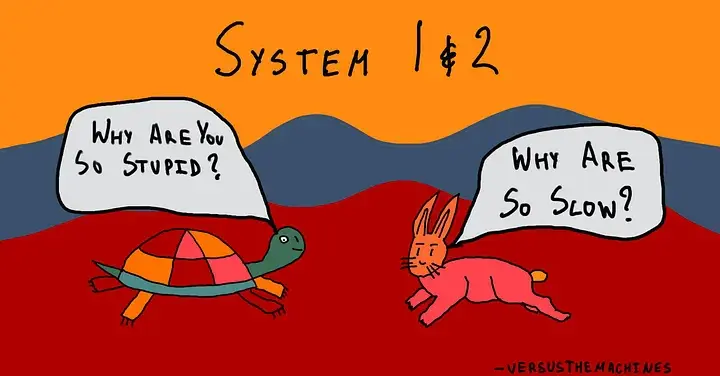
Daniel Kahneman spent decades studying how humans make decisions. His conclusion, laid out in Thinking, Fast and Slow, is that we don’t have one brain — we have two systems running in parallel:

System 1 is fast, automatic, instinctive. It pattern-matches. It reacts. It’s the part of you that catches a ball before you consciously decide to reach for it. It doesn’t deliberate — it fires.

System 2 is slow, deliberate, effortful. It’s the part of you that works through a logic puzzle, reads a contract, or plans a difficult conversation. It’s expensive — metabolically and cognitively. You can’t run it all day.

Most of cognition, Kahneman argues, is System 1. System 2 is reserved for when it counts.

The Third Layer Kahneman Didn’t Name

Neuroscience has a different framing — one that predates Kahneman and goes deeper.

Paul MacLean’s triune brain model describes three evolutionary layers:

The reptilian brain — brainstem and cerebellum. Pure survival. Reflexes, breathing, heart rate. No reasoning. Just reaction.

The mammalian brain — the limbic system. Emotion, memory, social bonding, creativity. The part of you that feels, connects, and imagines.

The human brain — the neocortex, especially the prefrontal cortex. Abstract reasoning, planning, language, deep thought. The thing that makes us distinctly us.

The interesting part: these layers don’t replace each other. They stack. They run in parallel. The neocortex doesn’t turn off the limbic system — it converses with it.

Three Models. Three Layers.

Here’s the theory:

Haiku is the reptilian brain.

Fast. Cheap. Reflexive. It pattern-matches and responds. It’s System 1 made silicon. You use Haiku for the things that need to happen instantly — classification, tagging, quick lookups, high-volume inference at the edge. It doesn’t deliberate. It fires.

Sonnet is the mammalian brain.

And this is where it gets interesting.

Sonnet is not the compromise between fast and slow. It’s something qualitatively different. The limbic system isn’t a weaker neocortex — it’s where creativity lives. Emotion. Connection. Flow.

Sonnet is where you go when you need to think with feeling. When the problem isn’t purely logical and it isn’t purely reflexive. When you’re writing, exploring, building, ideating. When you’re at 3am and something is trying to surface.

Opus is the neocortex.

Slow. Expensive. Deliberate. It reasons through problems that require holding multiple competing ideas in tension. You bring Opus when the stakes are high and the problem is genuinely hard — architecture decisions, legal analysis, long-horizon planning. It’s System 2. You can’t run it on everything; it costs too much.

Why This Matters for How You Work

If this model is right, the choice of which model to use isn’t just a cost-performance tradeoff. It’s a cognitive mode selection.

Routing a creative problem to Opus is like asking a team of senior engineers to brainstorm your product name. You’ll get a technically rigorous answer when you needed a generative one. You’ll get analysis when you needed flow.

Routing a complex architecture decision to Haiku is the inverse mistake — you’re asking your reflexes to do your planning.

The instinct to “always use the smartest model” misses this. Bigger isn’t always better. It’s about matching the cognitive mode to the task.

Model Brain Layer System Use Case
Haiku Brainstem / Cerebellum System 1 Extraction, tagging, classification, high-volume inference
Sonnet Limbic System Flow state Writing, coding, building, exploring, 3am crystallization
Opus Prefrontal Cortex System 2 Architecture, legal, long-horizon planning, high-stakes reasoning

A Note on the Naming

I don’t know if Anthropic intended this. The official explanation is capability tiers: Haiku is fastest and cheapest, Sonnet is balanced, Opus is most capable.

But the poetic forms map. The cognitive layers map. The systems map.

Maybe that’s coincidence. Maybe it’s the kind of thing that happens when a company thinks carefully about what they’re building.

The Practical Takeaway

Next time you open a new conversation, don’t default to Opus because it “feels safer.” Ask what mode you’re in:

  • Classifying, reacting, extracting at scale → Haiku
  • Creating, exploring, building, flowing → Sonnet
  • Reasoning through hard, high-stakes, complex problems → Opus

And if you find yourself reaching for Sonnet at 3am when something is trying to crystallize —

You already know why.

Written at 3:30am. First draft always beats the edited version.

— Rahul

I’m building knowledge-worker — a local-first knowledge graph that gives AI assistants durable, provenance-backed memory across sessions. If you’ve ever re-explained the same context to Claude three times in a week, it might be for you.