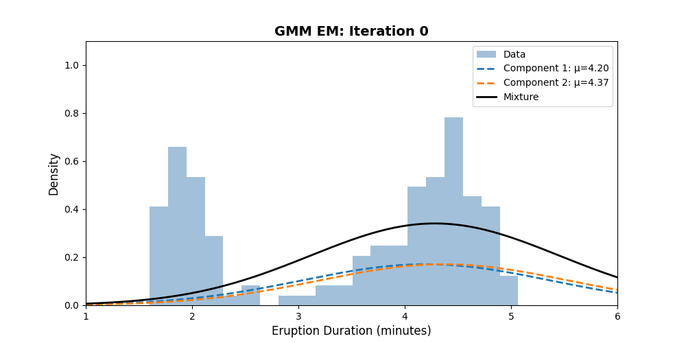
You have a dataset that clearly contains distinct groups, but nobody has labelled them. K-Means would give you hard boundaries — each point belongs to exactly one cluster. But what if a data point sits right between two clusters? Shouldn’t we express that uncertainty?
Gaussian Mixture Models (GMMs) do exactly this. They model your data as a mixture of Gaussian distributions, assigning each point a probability of belonging to each cluster — not a hard label. By the end of this post, you’ll implement a GMM from scratch using the EM algorithm and cluster real data from the Old Faithful geyser.
If you haven’t read the EM algorithm tutorial yet, don’t worry — we’ll explain everything you need here. But if you want the gentle coin-toss introduction first, start there.
Quick Win: Cluster Old Faithful Eruptions
Old Faithful is a geyser in Yellowstone National Park. Its eruptions come in two types: short (~2 min) with short waits, and long (~4.5 min) with long waits. Let’s discover these clusters automatically.

import numpy as np
import matplotlib.pyplot as plt

def gaussian_pdf(x, mu, sigma2):
    """Univariate Gaussian probability density function."""
    return (1 / np.sqrt(2 * np.pi * sigma2)) * np.exp(-0.5 * (x - mu)**2 / sigma2)

def fit_gmm(data, K=2, max_iter=50, tol=1e-6):
    """
    Fit a Gaussian Mixture Model using EM.

    Args:
        data: 1D array of observations
        K: number of mixture components
        max_iter: maximum EM iterations
        tol: convergence threshold

    Returns:
        means, variances, weights, responsibilities, log_likelihoods
    """
    N = len(data)

    # Initialise parameters
    rng = np.random.default_rng(42)
    means = rng.choice(data, K, replace=False)
    variances = np.full(K, np.var(data))
    weights = np.full(K, 1.0 / K)

    log_liks = []

    for iteration in range(max_iter):
        # E-STEP: Compute responsibilities
        resp = np.zeros((N, K))
        for k in range(K):
            resp[:, k] = weights[k] * gaussian_pdf(data, means[k], variances[k])
        resp /= resp.sum(axis=1, keepdims=True)

        # M-STEP: Update parameters
        Nk = resp.sum(axis=0)
        means = (resp * data[:, None]).sum(axis=0) / Nk
        variances = (resp * (data[:, None] - means)**2).sum(axis=0) / Nk
        weights = Nk / N

        # Compute log-likelihood
        ll = np.sum(np.log(sum(
            weights[k] * gaussian_pdf(data, means[k], variances[k])
            for k in range(K)
        )))
        log_liks.append(ll)

        if iteration > 0 and abs(log_liks[-1] - log_liks[-2]) < tol:
            break

    return means, variances, weights, resp, log_liks

# Old Faithful eruption durations
eruptions = np.array([
    3.6, 1.8, 3.333, 2.283, 4.533, 2.883, 4.7, 3.6, 1.95, 4.35,
    1.833, 3.917, 4.2, 1.75, 4.7, 2.167, 1.75, 4.8, 1.6, 4.25,
    1.8, 1.75, 3.45, 3.067, 4.533, 3.6, 1.967, 4.083, 3.85, 4.433,
    4.3, 4.467, 3.367, 4.033, 3.833, 2.017, 1.867, 4.833, 1.833, 4.783,
    4.35, 1.883, 4.567, 1.75, 4.533, 3.317, 3.833, 2.1, 4.633, 2.0,
    4.8, 4.716, 1.833, 4.833, 1.733, 4.883, 3.717, 1.667, 4.567, 4.317,
    2.233, 4.5, 1.75, 4.8, 1.817, 4.4, 4.167, 4.7, 2.067, 4.7,
    4.033, 1.967, 4.5, 4.0, 1.983, 5.067, 2.017, 4.567, 3.883, 3.6,
    4.133, 4.333, 4.1, 2.633, 4.067, 4.933, 3.95, 4.517, 2.167, 4.0,
    2.2, 4.333, 1.867, 4.817, 1.833, 4.3, 4.667, 3.75, 1.867, 4.9,
    2.483, 4.367, 2.1, 4.5, 4.05, 1.867, 4.583, 1.883, 4.367, 1.75,
    4.417, 1.967, 4.185, 1.883, 4.3, 1.767, 4.533, 2.35, 4.533, 4.45,
    3.567, 4.5, 4.15, 3.817, 3.917, 4.45, 2.0, 4.283, 4.767, 4.533,
    1.85, 4.25, 1.983, 2.25, 4.75, 4.117, 2.15, 4.417, 1.817, 4.467,
])

means, variances, weights, resp, log_liks = fit_gmm(eruptions)

print(f"Cluster 1: μ = {means[0]:.2f} min, σ = {np.sqrt(variances[0]):.2f}, weight = {weights[0]:.2f}")
print(f"Cluster 2: μ = {means[1]:.2f} min, σ = {np.sqrt(variances[1]):.2f}, weight = {weights[1]:.2f}")
The result: EM discovers two clear groups — short eruptions (~2.0 min, ~35% of data) and long eruptions (~4.3 min, ~65% of data). Let’s visualise:

x_plot = np.linspace(1, 6, 300)
mixture = sum(weights[k] * gaussian_pdf(x_plot, means[k], variances[k]) for k in range(2))

plt.figure(figsize=(10, 5))
plt.hist(eruptions, bins=20, density=True, alpha=0.5, color='steelblue', label='Data')
for k in range(2):
    component = weights[k] * gaussian_pdf(x_plot, means[k], variances[k])
    plt.plot(x_plot, component, '--', linewidth=2, label=f'Component {k+1}: μ={means[k]:.2f}')
plt.plot(x_plot, mixture, 'k-', linewidth=2, label='Mixture')
plt.xlabel('Eruption Duration (minutes)')
plt.ylabel('Density')
plt.title('GMM Fit to Old Faithful Eruption Data')
plt.legend()
plt.show()
What Just Happened?
A GMM assumes your data was generated by a process like this:
- Randomly pick one of
$K$ Gaussian components (with probabilities $pi_1, ldots, pi_K$)
- Draw a data point from that Gaussian
The catch: you observe the data points, but not which component generated each one. This hidden information — the component assignments — is the latent variable that EM handles.
E-Step: “Who Generated This Point?”
Given our current parameter estimates, we compute the responsibility of each component for each data point:

Think of $r_{nk}$ as “how much does component $k$ claim ownership of data point $x_n$?” If a point sits right at the mean of component 1 and far from component 2, then $r_{n1} approx 1$ and $r_{n2} approx 0$.
This is exactly the same idea as the soft assignments in the coin toss EM — instead of hard clustering, each point gets fractional membership.
# Let's trace the responsibilities for a few data points
print("Responsibilities (probability of belonging to each cluster):")
print(f"{'Duration':>10s}  {'Cluster 1':>10s}  {'Cluster 2':>10s}  {'Assignment':>12s}")
print("-" * 50)
for idx in [0, 1, 4, 7, 23]:
    dur = eruptions[idx]
    r1, r2 = resp[idx]
    label = "Short" if r1 > 0.5 else "Long"
    print(f"{dur:10.2f}  {r1:10.4f}  {r2:10.4f}  {label:>12s}")
M-Step: “Update the Gaussians”
Using the responsibilities as weights, we re-estimate each component’s parameters. The formulas are weighted maximum likelihood estimates — the same MLE you’d compute with complete data, but weighted by the responsibilities:
Effective number of points assigned to component $k$:

Updated mean (weighted average of data):

Updated variance (weighted variance):

Updated mixing weight:

Notice the pattern: if a point has $r_{nk} = 0.8$ for component $k$, then 80% of that point’s “mass” goes toward updating component $k$‘s parameters. This is exactly how weighted MLE works.
Convergence
Let’s verify that EM increases the log-likelihood at every step:
plt.figure(figsize=(8, 4))
plt.plot(range(1, len(log_liks) + 1), log_liks, 'g-o', markersize=6)
plt.xlabel('Iteration')
plt.ylabel('Log-Likelihood')
plt.title('EM Monotonically Increases the Log-Likelihood')
plt.grid(True, alpha=0.3)
plt.show()

Going Deeper
The Full GMM Log-Likelihood
The log-likelihood we’re maximising is:

The $log$ of a sum makes this hard to optimise directly — you can’t just take the derivative and set it to zero. That’s why we need EM: it transforms this intractable problem into a sequence of tractable weighted MLE problems.
Choosing K: How Many Clusters?
GMMs require you to specify the number of components $K$. Too few and you underfit; too many and you overfit. Common approaches:
BIC (Bayesian Information Criterion):

where $p$ is the number of parameters ($3K - 1$ for univariate GMMs: $K$ means + $K$ variances + $K-1$ weights).
def compute_bic(data, K_range=range(1, 6)):
    """Compute BIC for different numbers of components."""
    bics = []
    for K in K_range:
        means, variances, weights, _, log_liks = fit_gmm(data, K=K)
        n_params = 3 * K - 1
        bic = -2 * log_liks[-1] + n_params * np.log(len(data))
        bics.append(bic)
    return list(K_range), bics

K_values, bics = compute_bic(eruptions)
print("BIC scores:")
for k, bic in zip(K_values, bics):
    marker = " ← best" if bic == min(bics) else ""
    print(f"  K={k}: BIC = {bic:.1f}{marker}")
Lower BIC is better. For Old Faithful, $K=2$ should win clearly.
GMM vs K-Means
| Feature |
K-Means |
GMM |
| Assignments |
Hard (0 or 1) |
Soft (probabilities) |
| Cluster shape |
Spherical only |
Elliptical (with full covariance) |
| Uncertainty |
No |
Yes — $r_{nk}$ quantifies it |
| Output |
Cluster labels |
Full generative model |
| Speed |
Faster |
Slower (but more informative) |
K-Means is actually a special case of GMMs where all covariances are equal and small, forcing the responsibilities toward 0 or 1.
Common Pitfalls
-
Singularities — If a component collapses onto a single data point, its variance goes to zero and the likelihood goes to infinity. Fix: add a small floor to variances (e.g.,
$sigma^2 geq 10^{-6}$).
-
Initialisation sensitivity — Like all EM algorithms, GMMs can get stuck in local optima. Run multiple initialisations and keep the best result.
-
Label switching — The component labels are arbitrary. After fitting, component 1 in one run might correspond to component 2 in another.
-
High dimensions — In high dimensions, full covariance matrices have
$mathcal{O}(d^2)$ parameters per component. Use diagonal or tied covariances to reduce complexity.
When NOT to Use GMMs
-
Non-Gaussian clusters — If your clusters are banana-shaped or have complex geometry, GMMs will struggle. Consider DBSCAN or spectral clustering.
-
Very high dimensions — The curse of dimensionality makes density estimation unreliable. Reduce dimensions first (PCA, t-SNE).
-
Huge datasets — Full EM on millions of points is slow. Use mini-batch variants or the scikit-learn implementation.
Multivariate Extension
Our implementation handles 1D data. For $d$-dimensional data, the Gaussian PDF becomes:

The M-step updates become matrix operations, but the structure is identical: weighted means, weighted covariance matrices, updated mixing weights.
Deep Dive: The Paper
Dempster, Laird, and Rubin (1977)
The EM algorithm for GMMs is a specific instance of the general framework introduced by Dempster, A.P., Laird, N.M. and Rubin, D.B. (1977) “Maximum Likelihood from Incomplete Data via the EM Algorithm”, Journal of the Royal Statistical Society, Series B, 39(1), 1–38.
The paper unified a collection of ad-hoc algorithms that had been used in various fields — genetics, astronomy, engineering — under a single theoretical framework. Their key contribution was proving that every EM iteration is guaranteed to increase the likelihood (or leave it unchanged).
“Each iteration of a generalized EM algorithm increases the likelihood and the sequence of likelihood values converges.”
— Dempster, Laird & Rubin (1977)
The Complete-Data Framework
In GMM terms, the paper’s framework maps to:
-
Observed (incomplete) data
$X$: the data points $x_1, ldots, x_N$
-
Latent variables
$Z$: the component assignments $z_1, ldots, z_N$ (which Gaussian generated each point)
-
Complete data:
$(X, Z)$ — if we knew both, MLE would be trivial
-
Parameters
$theta = {mu_k, sigma_k^2, pi_k}$: what we want to estimate
The E-step computes $Q(theta mid theta^{(t)})$ — the expected complete-data log-likelihood:

The M-step maximises this over $theta$, yielding the weighted MLE formulas we derived earlier.
Bishop’s Modern Treatment
Bishop’s Pattern Recognition and Machine Learning (2006), Chapter 9 provides the most accessible modern treatment of GMMs. Key insights include:
-
GMMs as a density estimator — beyond clustering, GMMs give you a full probability model
$p(x)$ that you can sample from, evaluate, and use for anomaly detection
-
Relationship to K-Means — Bishop shows that K-Means is the zero-temperature limit of GMMs
-
Bayesian GMMs — placing priors on the parameters avoids singularities and enables automatic model selection. This connects to MCMC methods for posterior inference.
The Stanford EM Lecture
The original code in this tutorial references the Stanford Statistics 315a lecture notes on EM by Trevor Hastie and Rob Tibshirani. Slide 13 gives the GMM update equations we implemented.
Further Reading
-
Dempster, Laird & Rubin (1977) — The foundational EM paper
-
Bishop’s PRML, Chapter 9 — The clearest modern GMM treatment
-
Stanford EM Lecture Slides — Concise reference for the update equations
-
Scikit-learn GaussianMixture — Production-ready implementation with full covariance support
Try It Yourself
The interactive notebook includes exercises:
-
2D clustering — Extend the algorithm to cluster both eruption duration and waiting time simultaneously
-
Model selection — Plot BIC vs K and find the optimal number of components
-
Initialisation experiments — Run with 10 different random seeds and compare results
-
Compare with scikit-learn — Verify your implementation matches
sklearn.mixture.GaussianMixture
-
Anomaly detection — Use the fitted GMM to flag data points with low probability as outliers
Interactive Tools
-
Distribution Explorer — Visualise Gaussian and other distributions that form the components of mixture models
Related Posts
Frequently Asked Questions
What are responsibilities in a Gaussian Mixture Model?
Responsibilities are the probabilities that each data point belongs to each mixture component. During the E-step, the model computes how likely it is that component k generated data point n, given the current parameter estimates. These soft assignments sum to 1 across all components for each data point.
How does a GMM differ from simply running K-Means?
A GMM provides soft probabilistic assignments rather than hard labels, captures elliptical cluster shapes through full covariance matrices, and outputs a complete generative model you can sample from. K-Means only produces spherical cluster boundaries and gives no measure of uncertainty for points near cluster edges.
Why does the EM algorithm sometimes converge to a poor solution?
EM is guaranteed to increase the log-likelihood at every iteration, but it only finds a local maximum, not necessarily the global one. The final solution depends on the initial parameter values. Running EM multiple times with different random initialisations and selecting the result with the highest log-likelihood is the standard workaround.
What is the singularity problem in GMMs and how do I avoid it?
If a Gaussian component collapses onto a single data point, its variance approaches zero and the likelihood goes to infinity. This creates a degenerate solution. You can prevent this by adding a small floor to the variance (e.g., 1e-6), using regularisation, or placing a Bayesian prior on the covariance parameters.
How do I decide how many mixture components K to use?
The Bayesian Information Criterion (BIC) is the most common approach. Fit GMMs with different values of K, compute the BIC for each, and choose the K with the lowest BIC. The BIC balances model fit (log-likelihood) against complexity (number of parameters), penalising models that are unnecessarily complex.


 3 Nisan BİM aktüel teknoloji ürünleri arasında akülü Volvo kepçe, Renegade ATV, Range Rover jeep, Mercedes AMG, Chevrolet Camaro gibi araçlar yer alıyor.

 Hyundai’den Çinlilere ucuz SUV dersi! 6.200 dolarlık Hyundai Exter tanıtıldı! Ayrıca 607 km menziliyle elektrikli Toyota C-HR+, İsrail’in silahlarıyla anılan VW’den 2026 VW T-Roc ve Astra dizel