Introduction
Every report, dashboard, and visual in Power BI is only as good as the data model behind it. You can have perfect DAX measures and stunning visuals, but if your data model is poorly designed, your numbers will be wrong, your report will be slow, and your users will lose trust.
Data modeling is the process of organizing, structuring, and connecting your data tables so that Power BI can calculate results correctly and perform efficiently. It determines how tables relate to each other, how filters flow between them, and ultimately how every single number in your report is computed.
This article is a deep-dive into the core concepts of Power BI data modeling. We will cover SQL-style joins, Power BI relationships, fact and dimension tables, schema designs, and common pitfalls — all with real-life examples and clear guidance on where to perform each action in the Power BI interface.
Part 1: What Is Data Modeling?
Data modeling is the practice of defining how your data tables are structured and how they connect to one another. In Power BI specifically, a data model is the collection of all your tables, the relationships between them, and the calculated columns, measures, and hierarchies you build on top.
A well-designed data model achieves three goals:
-
Correctness — Filters propagate properly, so aggregations (SUM, COUNT, AVERAGE) return accurate results across related tables.
-
Performance — The VertiPaq engine can compress and query data efficiently, keeping report load times fast even at scale.
-
Simplicity — Report authors can drag and drop fields intuitively without needing to understand complex workarounds.
A poorly designed model, by contrast, leads to ambiguous relationships, inflated row counts, circular dependencies, and DAX formulas that become nightmarishly complex just to produce simple totals.
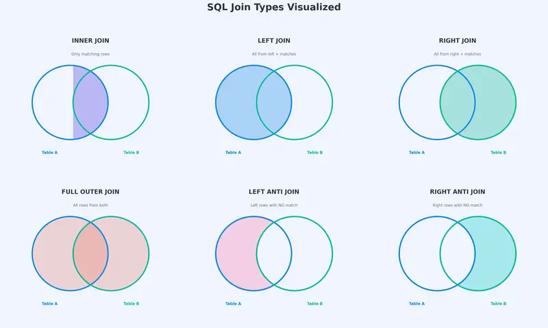
Part 2: SQL Joins — Combining Data Before It Enters the Model
Before data reaches your Power BI model, you often need to combine tables from one or more sources. This is where joins come in. Joins are operations that merge rows from two tables based on a matching condition (a common column). In Power BI, joins are performed in Power Query Editor (the data transformation layer), not in the model itself.

Think of a join as a question: “For each row in Table A, what matching rows exist in Table B?”
The answer depends on the type of join you use.
2.1 INNER JOIN
What it does: Returns only the rows where a match exists in both tables. If a row in Table A has no corresponding match in Table B, it is excluded — and vice versa.
Real-life example: You have an Orders table and a Customers table. An INNER JOIN on CustomerID returns only orders placed by customers who exist in the Customers table. If there is an order with a CustomerID that does not appear in Customers (perhaps an orphaned record), that order is dropped.
Orders Table              Customers Table
┌──────────┬────────┐     ┌──────────┬──────────┐
│ OrderID  │ CustID │     │ CustID   │ Name     │
├──────────┼────────┤     ├──────────┼──────────┤
│ 1001     │ C1     │     │ C1       │ Alice    │
│ 1002     │ C2     │     │ C2       │ Bob      │
│ 1003     │ C3     │     │ C4       │ Diana    │
│ 1004     │ C5     │     │ C5       │ Eve      │
└──────────┴────────┘     └──────────┴──────────┘

INNER JOIN Result (on CustID):
┌──────────┬────────┬──────────┐
│ OrderID  │ CustID │ Name     │
├──────────┼────────┼──────────┤
│ 1001     │ C1     │ Alice    │
│ 1002     │ C2     │ Bob      │
│ 1004     │ C5     │ Eve      │
└──────────┴────────┴──────────┘
→ Order 1003 (C3) is dropped: no match in Customers.
→ Customer C4 (Diana) is dropped: no match in Orders.

When to use it: When you only want records that exist in both tables and are comfortable discarding unmatched rows.
2.2 LEFT (OUTER) JOIN
What it does: Returns all rows from the left table (Table A), plus matching rows from the right table (Table B). If a row in the left table has no match, the right-side columns are filled with null.
Real-life example: You want a complete list of all orders, with customer names attached where available. Even if an order’s CustomerID has no match in Customers, you still want to see that order.
LEFT JOIN Result (Orders LEFT JOIN Customers on CustID):
┌──────────┬────────┬──────────┐
│ OrderID  │ CustID │ Name     │
├──────────┼────────┼──────────┤
│ 1001     │ C1     │ Alice    │
│ 1002     │ C2     │ Bob      │
│ 1003     │ C3     │ null     │  ← No match, but order is kept
│ 1004     │ C5     │ Eve      │
└──────────┴────────┴──────────┘
→ All 4 orders are preserved. Customer Diana (C4) has no order, so she does not appear.
When to use it: When the left table is your “primary” table and you want every row from it, enriched with optional data from the right table.
2.3 RIGHT (OUTER) JOIN
What it does: The mirror of a LEFT JOIN. Returns all rows from the right table, plus matching rows from the left table. Unmatched left-side columns are filled with null.
Real-life example: You want a list of all customers, with their orders attached where applicable. Customers with no orders still appear.
RIGHT JOIN Result (Orders RIGHT JOIN Customers on CustID):
┌──────────┬────────┬──────────┐
│ OrderID  │ CustID │ Name     │
├──────────┼────────┼──────────┤
│ 1001     │ C1     │ Alice    │
│ 1002     │ C2     │ Bob      │
│ null     │ C4     │ Diana    │  ← No order, but customer is kept
│ 1004     │ C5     │ Eve      │
└──────────┴────────┴──────────┘
→ Order 1003 (C3) is dropped because C3 is not in Customers.
When to use it: When the right table is your anchor. In practice, most analysts simply swap the table order and use a LEFT JOIN instead — both achieve the same result.
2.4 FULL OUTER JOIN
What it does: Returns all rows from both tables. Where a match exists, the columns are merged. Where no match exists on either side, the missing columns are filled with null.
Real-life example: You want to see every order and every customer, whether they match or not — useful for data reconciliation or finding orphaned records.
FULL OUTER JOIN Result:
┌──────────┬────────┬──────────┐
│ OrderID  │ CustID │ Name     │
├──────────┼────────┼──────────┤
│ 1001     │ C1     │ Alice    │
│ 1002     │ C2     │ Bob      │
│ 1003     │ C3     │ null     │  ← Order with no customer
│ null     │ C4     │ Diana    │  ← Customer with no order
│ 1004     │ C5     │ Eve      │
└──────────┴────────┴──────────┘
→ Nothing is dropped. Both unmatched sides are preserved.
When to use it: Data quality checks, reconciliation, or when you cannot afford to lose any records from either table.

2.5 LEFT ANTI JOIN
What it does: Returns only the rows from the left table that have NO match in the right table. It is the opposite of an INNER JOIN from the left table’s perspective.
Real-life example: You want to find orders that reference a CustomerID that does not exist in the Customers table — orphaned orders.
LEFT ANTI JOIN Result:
┌──────────┬────────┐
│ OrderID  │ CustID │
├──────────┼────────┤
│ 1003     │ C3     │  ← This order has no matching customer
└──────────┴────────┘
→ Only unmatched rows from the left table are returned.
When to use it: Finding orphaned or unmatched records. Data validation. Identifying gaps.
2.6 RIGHT ANTI JOIN
What it does: Returns only the rows from the right table that have NO match in the left table.
Real-life example: You want to find customers who have never placed an order.
RIGHT ANTI JOIN Result:
┌────────┬──────────┐
│ CustID │ Name     │
├────────┼──────────┤
│ C4     │ Diana    │  ← This customer has no orders
└────────┴──────────┘
→ Only unmatched rows from the right table are returned.
When to use it: Identifying inactive customers, unused products, or entities with no associated transactions.
2.7 How to Perform Joins in Power BI (Step-by-Step)
Joins in Power BI are performed in Power Query Editor, using the Merge Queries feature.
Step 1: Open Power BI Desktop and click Transform Data (on the Home ribbon) to enter Power Query Editor.
Step 2: Select the table you want to act as the “left” table in the Queries pane on the left.
Step 3: On the Home ribbon in Power Query Editor, click Merge Queries (or Merge Queries as New if you want a separate output table).
Step 4: In the Merge dialog:
- The top table is your left table (already selected).
- Select the bottom table (your right table) from the dropdown.
- Click on the matching column(s) in both table previews (e.g., CustID in both).
- At the bottom of the dialog, choose your Join Kind from the dropdown:
- Inner Join
- Left Outer (All from first, matching from second)
- Right Outer (All from second, matching from first)
- Full Outer (All rows from both)
- Left Anti (Rows only in first)
- Right Anti (Rows only in second)
Step 5: Click OK. A new column appears in your table containing the merged data as nested tables.
Step 6: Click the expand icon (↔) on the new column header to select which columns from the right table you want to bring in.
Step 7: Click Close & Apply to load the merged result into your data model.
Part 3: Power BI Relationships — Connecting Tables in the Model
While joins physically merge two tables into one (performed during data loading in Power Query), relationships are logical connections between separate tables that remain in your data model. They tell Power BI how to filter and aggregate data across tables without combining them.
This distinction is critical: joins happen before data enters the model; relationships exist within the model.
3.1 Cardinality Types
Cardinality defines how many rows in one table can match rows in another table.
One-to-Many (1:M) — The Gold Standard
The most common and recommended relationship type. One row in the “one” side matches zero, one, or many rows on the “many” side.
Example: One row in Customers (CustomerID = C1) can match many rows in Orders (multiple orders placed by C1). But each order has exactly one customer.
Customers (1 side)          Orders (Many side)
┌────────┬────────┐         ┌──────────┬────────┬────────┐
│ CustID │ Name   │         │ OrderID  │ CustID │ Amount │
├────────┼────────┤         ├──────────┼────────┼────────┤
│ C1     │ Alice  │───1:M──▶│ 1001     │ C1     │ 50     │
│        │        │         │ 1005     │ C1     │ 120    │
│ C2     │ Bob    │───1:M──▶│ 1002     │ C2     │ 80     │
└────────┴────────┘         └──────────┴────────┴────────┘
Why it is preferred: Filters flow cleanly from the “one” side to the “many” side. When you select “Alice” in a slicer, Power BI filters the Orders table to only show Alice’s orders. Aggregations (SUM of Amount) work correctly and unambiguously.
Many-to-Many (M:M)
Multiple rows on both sides can match each other. This occurs when neither table has unique values in the join column.
Example: A Students table and a Courses table connected through a bridge table, where each student takes multiple courses and each course has multiple students. If you connect Students directly to Courses without a bridge table, you get an M:M relationship.
Risks: M:M relationships can produce unexpected results because filters can flow in ways that cause double-counting or inflated totals. Power BI allows them, but they should be used cautiously and are often a sign that a bridge table (a fact table representing the enrollment) is needed.
One-to-One (1:1)
Each row in Table A matches exactly one row in Table B. Both columns in the relationship contain unique values.
Example: An Employees table and an EmployeeDetails table, where each employee has exactly one detail record.
When it arises: Usually when a single table has been split into two for organizational reasons (e.g., separating PII data from non-PII data). Consider whether the tables should simply be merged.
3.2 Cross-Filter Direction
Cross-filter direction controls how slicer and filter selections propagate between related tables.
Single Direction (Default for 1:M)
Filters flow from the “one” side to the “many” side only. This is the default and recommended setting.
Customers ──filter──▶ Orders
(Selecting a customer filters their orders)

Orders ──X──▶ Customers
(Selecting an order does NOT filter the Customers table by default)
Why single is preferred: It keeps filter behavior predictable. Report authors know that dimension tables filter fact tables, and not the other way around.
Both Directions (Bidirectional)
Filters flow in both directions. Selecting a value in either table filters the other.
Customers ◀──filter──▶ Orders
When to use: Rarely. Sometimes necessary when you have a bridge table in an M:M scenario and need filters to propagate through it. Bidirectional filtering can cause performance issues and ambiguous filter contexts if overused.
Recommendation: Start with single-direction filtering. Only switch to bidirectional when you have a specific, well-understood reason.
3.3 Active vs. Inactive Relationships
Power BI allows only one active relationship between any two tables at a time. If your data has multiple logical connections between the same two tables, you must designate one as active and the rest as inactive.
Example: A Sales table has both an OrderDate and a ShipDate column. Both logically connect to a Calendar table. You can create two relationships (OrderDate→Calendar and ShipDate→Calendar), but only one can be active.
Calendar (Date)
    │
    ├── Active Relationship ──── Sales[OrderDate]
    │
    └── Inactive Relationship ─ ─ ─ Sales[ShipDate]  (dashed line in Model View)
The active relationship is used by default in all DAX calculations. To use the inactive relationship, you invoke the USERELATIONSHIP function:
Ship Date Sales =
CALCULATE(
    SUM(Sales[Amount]),
    USERELATIONSHIP(Sales[ShipDate], Calendar[Date])
)
This concept directly connects to role-playing dimensions, discussed later in this article.
3.4 How to Create and Manage Relationships in Power BI (Step-by-Step)
Method 1: Model View (Drag-and-Drop)
Step 1: In Power BI Desktop, click the Model View icon on the left sidebar (the icon with three connected boxes).
Step 2: You will see all your tables displayed as boxes with their columns listed.
Step 3: To create a relationship, click on a column in one table and drag it to the matching column in another table. A line appears connecting the two tables.
Step 4: Power BI will auto-detect the cardinality and cross-filter direction. Double-click the relationship line to edit these properties.
Method 2: Manage Relationships Dialog
Step 1: Go to the Home ribbon (or Modeling ribbon) and click Manage Relationships.
Step 2: A dialog appears showing all existing relationships. Click New to create one.
Step 3: Select the two tables and the matching columns from dropdowns.
Step 4: Set the cardinality (One-to-Many, Many-to-Many, One-to-One).
Step 5: Set the cross-filter direction (Single or Both).
Step 6: Check or uncheck Make this relationship active.
Step 7: Click OK to save.
Method 3: Auto-Detect
When you first load data, Power BI attempts to auto-detect relationships based on column names and data types. This works well for simple models but should always be reviewed manually. Go to Manage Relationships to verify what Power BI created and correct any mistakes.
Part 4: Joins vs. Relationships — What Is the Difference?

This is one of the most common points of confusion for Power BI beginners.
| Aspect |
Joins (Power Query) |
Relationships (Model) |
| Where |
Power Query Editor (Transform Data) |
Model View / Manage Relationships |
| When |
During data loading/transformation |
After data is loaded into the model |
| Result |
Physically merges two tables into one |
Keeps tables separate, connected logically |
| Row count |
Output table may have more or fewer rows |
Tables retain their original row counts |
| Use case |
Enriching/cleaning data before modeling |
Enabling cross-table filtering and aggregation |
| Performance |
Increases table size (more columns per row) |
Efficient — VertiPaq handles relationships natively |
| DAX impact |
Merged columns become part of one table |
DAX uses RELATED/RELATEDTABLE to traverse |
Rule of thumb: Use joins (Merge in Power Query) when you need to physically combine or clean data, such as adding a lookup column or deduplicating. Use relationships when you want to keep tables separate and let Power BI handle filtering and aggregation — which is the case for the vast majority of your model.
Part 5: Fact Tables vs. Dimension Tables
The foundation of any good data model is the separation of data into fact tables and dimension tables.
Fact Tables
A fact table stores the events or transactions of your business. Each row represents something that happened: a sale, a shipment, a click, a support ticket.
Characteristics of fact tables:
- Contain measures — numeric values you want to aggregate (Amount, Quantity, Cost, Duration).
- Contain foreign keys — columns that reference dimension tables (CustomerID, ProductID, DateKey).
- Tend to be tall (many rows, relatively few columns).
- Grow over time as new transactions occur.
Examples: Sales, Orders, WebClicks, SupportTickets, Shipments, FinancialTransactions.
Dimension Tables
A dimension table stores the descriptive attributes that provide context to your facts. They answer the “who, what, where, when, why” questions about your transactions.
Characteristics of dimension tables:
- Contain descriptive columns — names, categories, addresses, dates, hierarchies.
- Contain a primary key — a unique identifier for each row (CustomerID, ProductID, Date).
- Tend to be wide (many columns, relatively few rows compared to fact tables).
- Change slowly or infrequently.
Examples: Customers, Products, Calendar/Date, Geography, Employees, Stores.
How They Connect
┌──────────────┐     ┌──────────────────────────────┐     ┌──────────────┐
│  Customers   │     │         Sales (Fact)          │     │   Products   │
│  (Dimension) │     │                               │     │  (Dimension) │
├──────────────┤     ├──────────────────────────────┤     ├──────────────┤
│ *CustomerID  │◀─1:M│ SaleID                        │M:1─▶│ *ProductID   │
│  Name        │     │ CustomerID (FK)               │     │  ProductName │
│  City        │     │ ProductID (FK)                │     │  Category    │
│  Segment     │     │ DateKey (FK)                  │     │  Price       │
└──────────────┘     │ Quantity                      │     └──────────────┘
                     │ Amount                        │
                     └──────────────────────────────┘
                                   │
                                  M:1
                                   │
                              ┌─────────┐
                              │Calendar │
                              │(Dim)    │
                              ├─────────┤
                              │*Date    │
                              │ Month   │
                              │ Quarter │
                              │ Year    │
                              └─────────┘
The asterisk (*) denotes the primary key. Arrows show the “one” side pointing to the “many” side. Filters flow from dimensions into the fact table, which is exactly what you want — selecting a customer, product, or date filters the relevant sales.
Part 6: Schema Designs
A schema is the overall shape or architecture of your data model — how fact and dimension tables are arranged and connected.
6.1 Star Schema
The star schema is the recommended design for Power BI. It consists of a central fact table surrounded by dimension tables, each directly connected to the fact table. When visualized in Model View, the layout resembles a star.

                    ┌────────────┐
                    │  Calendar  │
                    └──────┬─────┘
                           │
┌────────────┐    ┌────────┴────────┐    ┌────────────┐
│ Customers  ├────┤   Sales (Fact)  ├────┤  Products  │
└────────────┘    └────────┬────────┘    └────────────┘
                           │
                    ┌──────┴─────┐
                    │   Stores   │
                    └────────────┘
Characteristics:
- One fact table at the center.
- Dimension tables connect directly to the fact table (one hop).
- Dimensions are denormalized — all descriptive attributes are in a single table per dimension, even if that means some redundancy.
Example: A Products dimension contains ProductName, SubCategory, Category, and Department all in one table, even though SubCategory→Category→Department is a hierarchy. The redundancy is intentional — it simplifies the model.
Advantages:
- Simple and intuitive for report authors.
- Power BI’s VertiPaq engine is optimized for star schemas.
- Filters travel one hop from dimension to fact — fast and predictable.
- DAX formulas are straightforward.
When to use: Almost always. This should be your default schema design in Power BI.
6.2 Snowflake Schema
A snowflake schema is a star schema where one or more dimension tables are normalized — broken into sub-tables connected in a chain.
┌──────────────┐    ┌──────────────┐    ┌──────────────────┐
│  Department  ├────┤  Category    ├────┤    Products      │
└──────────────┘    └──────────────┘    └────────┬─────────┘
                                                 │
                                        ┌────────┴────────┐
                                        │  Sales (Fact)   │
                                        └────────┬────────┘
                                                 │
                                          ┌──────┴─────┐
                                          │  Calendar  │
                                          └────────────┘
Instead of one Products dimension with all attributes, the snowflake breaks it into Products → Category → Department, each as a separate table.
Characteristics:
- Normalized dimension chains (multiple hops from fact to outermost dimension).
- Less data redundancy in dimension tables.
- More tables and relationships to manage.
Advantages:
- Reduced storage for dimension data (relevant in traditional data warehouses).
- Cleaner structure if dimensions are very large and highly hierarchical.
Disadvantages in Power BI:
- Filters must travel through multiple relationships to reach the fact table, which can complicate DAX and reduce performance.
- Report authors have to understand which sub-table contains which attribute.
- VertiPaq already compresses data extremely well, so the storage savings of normalization are negligible.
When to use: Rarely in Power BI. If your source data arrives snowflaked, consider flattening (denormalizing) the dimension chains in Power Query before loading them into the model. The result: a star schema.

6.3 Flat Table (Denormalized / DLAT)
A flat table model consists of a single, wide table that contains everything — facts and dimensions combined into one table.
┌─────────────────────────────────────────────────────────┐
│                   FlatSalesTable                        │
├─────────────────────────────────────────────────────────┤
│ SaleID │ Date │ CustomerName │ City │ ProductName │ ... │
│ Amount │ Quantity │ Category │ Segment │ StoreName │ ... │
└─────────────────────────────────────────────────────────┘
(One massive table — no relationships needed)
Characteristics:
- Everything in one table.
- No relationships because there is only one table.
- Extremely wide (many columns) and potentially very tall (many rows with repeated descriptive data).
Advantages:
- Simple for very small datasets or quick ad-hoc analysis.
- No relationships to configure.
- Easy to create from a single CSV or Excel export.
Disadvantages:
- Massive data redundancy (customer name, city, segment repeated on every row).
- Poor compression and large model size.
- No clear separation of measures vs. attributes.
- Difficult to maintain and extend.
- DAX calculations can behave unexpectedly because there is no clear filter direction.
When to use: Only for quick prototypes, small personal datasets, or when you genuinely have a single flat data source with fewer than a few thousand rows and no plans to scale.
6.4 Schema Comparison Summary
| Criteria |
Star Schema |
Snowflake Schema |
Flat Table |
| Complexity |
Low |
Medium-High |
Lowest |
| Performance in Power BI |
Best |
Good (but extra hops) |
Poor at scale |
| Data redundancy |
Moderate (in dimensions) |
Low |
Very high |
| Ease of DAX |
Easiest |
Harder (multi-hop) |
Unpredictable |
| Scalability |
Excellent |
Good |
Poor |
| Recommended for Power BI |
Yes — default choice |
Flatten if possible |
Small/ad-hoc only |

Part 7: Role-Playing Dimensions
A role-playing dimension is a single dimension table that serves multiple analytical purposes by connecting to the same fact table through different columns.
The most common example is the Calendar/Date dimension. A Sales fact table might have:
-
OrderDate — when the order was placed.
-
ShipDate — when the order was shipped.
-
DeliveryDate — when the order was delivered.
All three columns connect to the same Calendar table, but each represents a different analytical “role.”

How to Handle This in Power BI
Option A: One Calendar Table, Multiple Relationships
Create one Calendar table and establish three relationships to Sales. Designate one as active (typically OrderDate) and the others as inactive. Use USERELATIONSHIP in DAX when you need the inactive relationships:
Shipped Amount =
CALCULATE(
    SUM(Sales[Amount]),
    USERELATIONSHIP(Sales[ShipDate], Calendar[Date])
)
Pros: Single calendar table to maintain. Less data duplication.
Cons: Requires DAX knowledge for inactive relationships. Only one relationship is active for default behavior.
Option B: Duplicate Calendar Tables
Create separate calendar tables in Power Query (e.g., OrderCalendar, ShipCalendar, DeliveryCalendar), each with an active relationship to the respective date column. This means duplicating the Calendar table logic.
Pros: All relationships are active. No USERELATIONSHIP needed. Slicers can be placed on any calendar independently.
Cons: Multiple copies of the same data. More tables in the model.
Which to choose: Option A is cleaner for models where the non-primary date roles are used infrequently. Option B is better when all date roles are equally important and frequently sliced on.
Part 8: Common Data Modeling Issues and How to Avoid Them
Issue 1: Ambiguous Relationships
Symptom: Power BI shows an error: “A relationship already exists between these tables” or “Ambiguous paths.”
Cause: Multiple active relationship paths exist between two tables, and Power BI does not know which to use.
Fix: Ensure only one active relationship exists between any pair of tables. Use inactive relationships with USERELATIONSHIP for alternate paths.
Issue 2: Circular Dependencies
Symptom: Power BI warns about circular dependencies or refuses to create a relationship.
Cause: The relationships form a closed loop (A→B→C→A), and Power BI cannot determine a clear filter direction.
Fix: Restructure your model to eliminate the loop. Often this means consolidating tables or removing a redundant relationship.
Issue 3: Many-to-Many Without a Bridge Table
Symptom: Aggregations return inflated or incorrect totals.
Cause: Two tables are connected M:M directly because neither has unique values in the join column. Filters propagate ambiguously.
Fix: Introduce a bridge (junction/associative) table that contains one row for each valid combination, turning the M:M into two 1:M relationships.
Before (problematic):
Students ──M:M──▶ Courses

After (correct):
Students ──1:M──▶ Enrollments ◀──M:1── Courses
Issue 4: Using Bidirectional Filtering Everywhere
Symptom: Unexpected filter behavior, slow performance, or filters appearing to “leak” across unrelated parts of the model.
Cause: Cross-filter direction set to “Both” on many relationships.
Fix: Reset all relationships to single-direction (default). Only enable bidirectional where absolutely necessary and test the impact thoroughly.
Issue 5: Too Many Columns in Fact Tables
Symptom: Large model size, slow refresh, poor compression.
Cause: Descriptive columns (customer names, product categories, addresses) stored directly in the fact table instead of in dimension tables.
Fix: Move descriptive attributes to their own dimension tables. Keep only keys and measures in the fact table. Use Power Query to split data during loading.
Issue 6: Missing or Incorrect Date Table
Symptom: Time intelligence functions (TOTALYTD, SAMEPERIODLASTYEAR, etc.) do not work or return errors.
Cause: No proper date/calendar dimension exists, or the date column has gaps.
Fix: Create a dedicated Calendar table that covers the full date range of your data with no gaps. Mark it as a Date Table in Power BI (select the table → Modeling ribbon → Mark as Date Table). Ensure it has a column of data type Date with unique, contiguous values.
Part 9: Putting It All Together — A Modeling Workflow
Here is a practical workflow for building a clean Power BI data model:
Step 1: Understand the business questions. What do stakeholders need to analyze? (Revenue by region? Inventory by warehouse? Support tickets by priority?) The answers determine which facts and dimensions you need.
Step 2: Identify fact and dimension tables. Facts are the measurable events. Dimensions are the descriptive context. Separate them clearly.
Step 3: Clean and transform in Power Query. Use joins (Merge) to enrich data during loading. Flatten snowflaked dimensions. Remove unnecessary columns. Set correct data types.
Step 4: Load into the model and build relationships. Switch to Model View. Create 1:M relationships between dimension tables (one side) and fact tables (many side). Set cross-filter direction to single.
Step 5: Organize for usability. Hide foreign key columns from the report view (right-click → Hide in Report View). Create display folders. Add descriptions to key columns and measures. Arrange tables in a star layout in Model View.
Step 6: Build measures and test. Write DAX measures (SUM, AVERAGE, CALCULATE, etc.) and verify they return correct results. Test slicers to confirm filters propagate as expected.
Step 7: Optimize. Remove unused columns. Check model size. Profile query performance. Ensure date tables are properly marked.
Conclusion
Data modeling is not a step you rush through on the way to building visuals — it is the structural foundation that determines whether your Power BI reports are fast, accurate, and maintainable.
The key takeaways from this article:
-
Joins merge tables physically during data loading and are performed in Power Query. Use them for enrichment and cleanup.
-
Relationships connect tables logically within the model and enable cross-table filtering. They are the backbone of your data model.
-
Star schemas are the gold standard for Power BI. Keep fact tables at the center, surrounded by denormalized dimension tables.
-
Cardinality should be 1:M wherever possible. Avoid M:M unless you have a proper bridge table.
-
Cross-filter direction should default to single. Use bidirectional filtering sparingly and deliberately.
-
Role-playing dimensions handle scenarios where one dimension serves multiple analytical roles (e.g., multiple dates).
-
Common issues like ambiguous relationships, circular dependencies, and misplaced columns are almost always solvable by restructuring toward a clean star schema.
Invest time in your data model. Every minute spent designing a clean model saves hours of debugging DAX formulas and explaining incorrect numbers later.
This article is intended as a reference guide for Power BI practitioners at all levels. Bookmark it, share it with your team, and revisit it whenever you start a new project.




 Samsung’un özellikle Galaxy S26 Ultra modelinde yaygın olarak ekran sorunları yaşanıyor. Şirket, yakında serideki tüm telefonlar için sorunları çözecek bir güncelleme yayınlayacağını söyledi.