The 15-Millisecond AI: Building “Pre-Cognitive” Edge Caching on AWS

frist image

If you want to watch a product manager’s soul leave their body, sit in on a live demo of a Generative AI feature where the model takes 12 seconds to generate a response.

Typing… typing… typing…

In the world of AI product development, latency is the ultimate UX killer. You can have the smartest prompt and the most expensive foundational model in the world, but if your users have to stare at a spinning loading wheel for 10 seconds every time they click a button, they will abandon your app.

Most engineering teams try to solve this by streaming tokens to the frontend or switching to smaller, less capable models. But as a cloud architect, I prefer a different approach.

What if we stopped waiting for the user to ask the question?

What if we used the user’s application state to predict what they are going to ask, generated the answer in the background, and pushed it to a CDN edge location before their mouse even hovers over the button?

When I sketch this out for engineering leaders, the reaction is almost always the same: “Wait, we can pre-generate AI responses in the background and cache them at the CDN level to completely bypass inference latency?”

Yes. Here is how to build a “Pre-Cognitive” AI architecture using AWS Step Functions, Amazon Bedrock, and Amazon CloudFront with Lambda@Edge.

The Concept: From Reactive AI to Proactive Caching

Think about your favorite SaaS dashboard. When a user logs in on Monday morning, their “next best actions” are highly predictable.

  • They are going to ask for a summary of weekend alerts.
  • They are going to ask for the status of their latest deployment.
  • They are going to ask for a draft reply to their most urgent ticket.

Instead of waiting for the user to click “Summarize Alerts” and forcing them to wait 8 seconds for an LLM to read the data, we move the LLM inference out of the synchronous request path and into an asynchronous background job.

We generate the responses, store them as key-value pairs, and push them to the network edge. When the user finally clicks the button, the response loads in 15 milliseconds. It feels like magic.

The Architecture: Phase 1 (Background Generation)

To make this work without slowing down the initial user login, we decouple the generation using an event-driven flow.

frist image

1. The Trigger: When the user logs in (or enters a specific workflow), your backend fires an event to AWS EventBridge.
2. The Orchestrator: AWS Step Functions takes over. It acts as the background traffic cop, ensuring your API doesn’t hang.
3. The Inference: A Lambda function analyzes the user’s state, grabs the required context, and fires off 3 concurrent prompts to Amazon Bedrock (using a fast, cheap model like Claude 3 Haiku).
4. The Edge Push: Once Bedrock returns the generated text, Lambda pushes these pre-computed AI responses into Amazon CloudFront KeyValueStore (a globally distributed datastore designed specifically for edge functions) keyed by UserID_ActionID.

The Architecture: Phase 2 (The 15ms Delivery)

Now, the user is looking at their dashboard. They see a button that says “✨ Generate Morning Briefing.” They click it.

Because we are using CloudFront and Lambda@Edge (or CloudFront Functions), the request never even reaches your primary backend servers in us-east-1.

second video

1. The Interception: The user’s HTTPS request hits the closest AWS Edge location (e.g., a server in London, Tokyo, or New York). Lambda@Edge intercepts the request.
2. The Edge Lookup: Lambda@Edge checks the attached CloudFront KeyValueStore for the user’s pre-generated response.
3. Instant Delivery: If the response is there, it is returned instantly. The user experiences sub-20ms latency for a complex Generative AI task.
4. The Fallback: If the user asks a completely custom question that we didn’t predict, Lambda@Edge simply forwards the request to your standard API Gateway/Bedrock backend to generate the response synchronously.

The CTO Perspective: Tradeoffs and Reality Checks

As a technology strategist, I will be the first to tell you that “magic” always comes with an engineering invoice. You should only use this pattern if you understand the tradeoffs.

1. The Cost of Wasted Compute

By predicting 3 things the user might ask, you are generating tokens that might never be read. You are trading compute cost for user experience.
The Mitigation: Only use this pattern with ultra-cheap, highly efficient models like Claude 3 Haiku or Llama 3 8B. Do not use Claude 3 Opus or GPT-4o for speculative background generation, or you will torch your AWS bill.

2. State Invalidation

What happens if you pre-generate a “Deployment Summary” at 9:00 AM, but at 9:05 AM a deployment fails, and the user clicks the button at 9:06 AM? The cached AI response is now lying to them.
The Mitigation: Tie your cache invalidation to your application’s critical state changes. If a critical DB row updates, fire an EventBridge rule that immediately deletes the stale key from the CloudFront KeyValueStore.

3. Build Complexity vs. Product Value

Don’t build this for a general-purpose chatbox. Humans are too unpredictable. Build this for highly structured, high-value UX checkpoints—like daily briefings, code review summaries, or personalized dashboard greetings.

The Bottom Line

When we build AI applications, we often forget that the rules of distributed systems still apply. You don’t have to accept the latency of a foundational model as a fixed constraint.

By aggressively predicting user intent and leveraging AWS edge networking primitives like CloudFront and Lambda@Edge, you can completely mask LLM latency.

It takes your application from feeling like a “cool AI wrapper” to feeling like a deeply integrated, hyper-responsive superpower.

Have you struggled with GenAI latency in your production applications? Are you using streaming, or have you started exploring asynchronous generation? Let me know your architecture in the comments below.

Your Data Access Layer Doen’t Understand Databases

Here’s what nobody in the data access space wants to admit: the tools built to simplify database work have quietly offloaded the hardest parts back onto your application. Not by accident — by design. They model a pleasant fiction of what a database is, and when reality diverges, you pay for it in conditionals, workarounds, retries, and production incidents.

This is not a complaint about generated SQL. SQL quality is a separate argument, and an old one. The problem runs deeper.

Connection behavior is not a performance concern. It is a correctness concern.

Most data access layers don’t model that. Your application does — in feature flags, special cases, and debugging sessions you didn’t budget for.

Connection lifetime, concurrency, and identity are not independent concerns. They are the database.

Not all databases are the same machine

Most data access libraries are built around one mental model:

  • The server is already running
  • You connect
  • You execute commands
  • You commit or roll back
  • You disconnect
  • The server waits for the next client

SQL Server, PostgreSQL, Oracle, and MySQL broadly fit that model. For those databases, the standard approach works well enough that the cracks stay hidden for a while.

But not every database works that way.

In-memory embedded databases

SQLite and DuckDB in :memory: mode have a fundamental behavioral difference that most abstractions ignore entirely: the database is the connection.

Open one connection, you have a database. Open a second connection, you don’t get another connection to the same database. You get a different database. Empty. Gone.

That’s not a quirk. That’s the operational model.

A library built around “open and close connections freely per operation” will silently destroy your in-memory database between calls. No error. No warning. Just an empty database where your data used to be.

File-based embedded databases

File-based SQLite and DuckDB are not miniature SQL Servers. Their write behavior is fundamentally different:

  • One writer at a time, enforced at the engine level
  • Concurrent write attempts result in lock contention, busy timeouts, and failures
  • The journal mode and transaction settings interact with connection behavior in ways that bite you if you get them wrong

The standard advice — “open a connection, run a command, close it, repeat” — actively works against you here. Under concurrent load you’ll see lock errors. Under sequential load you’ll see busy timeouts. The “simple” connection pattern creates exactly the contention the database can’t handle.

This is so commonly mishandled that most dedicated SQLite tooling gets it wrong too.

LocalDB

Microsoft’s LocalDB was a genuinely good idea: full SQL Server semantics, no server install, attach a file and go. Great for local development and testing.

Until idle unload enters the picture.

If no connection is held for a configurable period, LocalDB unloads the database. Not an error — an unload. Your next operation reconnects and reattaches, which adds latency and can cause failures during test runs where operations are spaced out.

The fix is a sentinel connection: one persistent connection held open specifically to prevent idle unload. Not for running queries. Just to keep the database alive.

No mainstream data access library models this. You find out about it from a Stack Overflow answer at 11pm.

What the libraries actually do

This is not speculation. Here’s what each major option in the .NET ecosystem actually models.

Entity Framework Core opens and closes connections per query and per SaveChanges() call by default. It delegates pooling entirely to the ADO.NET provider — EF has no awareness of pool pressure or saturation. When you use an in-memory SQLite database with EF, the official workaround documented by Microsoft is to manually open the connection on the DbContext and hold it open for the lifetime of the context. The developer absorbs the problem the library doesn’t solve. There is no connection policy. There is a workaround in the docs.

NHibernate ties connection lifetime to the ISession. It has a more explicit unit-of-work model than EF, which helps with some lifetime issues, but the underlying assumption is unchanged: stable, server-style backend, many connections available, connection lifetime is a performance concern. No single-writer enforcement, no keepalive, no concept of connection-bound database identity.

Dapper doesn’t touch connection lifetime at all. You open it, you pass it in, Dapper runs the command, you close it. That’s the design — deliberately minimal. It’s not a flaw in Dapper. But it means connection policy is 100% on the caller, every time, with no structure and no guardrails.

Raw ADO.NET is the same. The documented guidance is to use using blocks and dispose promptly. That’s the policy: a coding convention. Not a library feature, not an enforced invariant — a convention you either follow or don’t.

None of them model connection policy as a function of database behavior. They model lifetime. They do not model constraints. Connection policy is either delegated to the provider, left to convention, or documented as a workaround.

The connection-per-command trap

Standard advice across almost every data access library is “use one connection per command.” Open, execute, consume results, close. Your DBA will approve. Your server database will be healthier.

That advice has real merit for server databases. It reduces leaks. It shortens connection lifetime. It keeps the pool healthy under normal load.

But follow it everywhere and you create three new problems:

You can’t use in-memory databases for testing. One connection per command means a new empty database on every operation. Your tests pass against nothing.

File-based embedded databases become unreliable. The write serialization problem doesn’t go away because you’re closing connections quickly — it gets worse, because you’re now racing to reacquire write locks constantly.

LocalDB unloads between operations. No persistent connection means no sentinel. Your test suite reconnects and reattaches on every run. Or fails partway through when the unload window closes before your next operation.

So you add feature flags. Database-specific code paths. If-SQLite-do-this, if-LocalDB-do-that. Your business logic now contains your database topology.

That is the abstraction failing at its core job.

Pool saturation: when “doing it right” still breaks

Say you got through all of the above. Feature flags in place. Connection handling tuned per database type. DBA is satisfied, cloud bill is down, everything works.

Then you get a traffic spike.

Requests pile up. Each one opens a connection. The pool has a maximum size — every pool does. Requests start waiting. Wait times compound. At this point you don’t get slow queries — you get connection acquisition failures. SQL Server throws Timeout expired. The timeout period elapsed prior to obtaining a connection from the pool. PostgreSQL reports remaining connection slots are reserved. SQLite escalates busy errors into lock failures.

You need something that governs connections. Not just “open and close promptly” — actual enforcement: when the pool is full, make everything else wait. Bounded concurrency tied to pool size, not just etiquette.

None of the libraries above have this. ADO.NET pooling will queue and timeout, but it doesn’t expose the control surface you need to shape behavior under load. You find out your limits when production hits them.

What you actually need: routing by intent

Databases already differentiate reads and writes. Your access layer doesn’t.

That missing distinction has consequences. If the layer exposed it, it could enforce:

  • Read-only sessions routed to a read replica, drawing from a separate pool
  • Write operations serialized where the database requires it
  • Each pool governed independently, sized to its workload
  • For embedded databases, the write limit set to one — enforced by the layer, not scattered across application code

This isn’t new capability. It’s the modeling that’s missing. Databases have always had these constraints. The access layer just never encoded them.

What modeling it correctly looks like

Connection behavior is a property of the database. It belongs in the data access layer, encoded explicitly, not left to convention or absorbed by the application.

Here’s what that looks like in practice. pengdows.crud exposes connection policy as a first-class configuration decision through DbMode:

Mode What it does When to use it
Standard Pool per operation, open late, close early Server databases: SQL Server, PostgreSQL, Oracle, MySQL
KeepAlive Holds a sentinel connection to prevent idle unload LocalDB
SingleWriter Many concurrent readers, one serialized writer File-based SQLite, file-based DuckDB
SingleConnection One connection, period In-memory :memory: databases
Best Auto-selects the correct mode based on database type When you want the right answer without thinking about it

Best maps automatically: SQLite/DuckDB :memory: gets SingleConnection; file-based SQLite/DuckDB gets SingleWriter; LocalDB gets KeepAlive; everything else gets Standard.

Configuration looks like this:

// File-based SQLite — enforces single writer, concurrent readers
new DatabaseContext(
    new DatabaseContextConfiguration { ConnectionString = connStr, DbMode = DbMode.SingleWriter },
    SqliteFactory.Instance);

// Or let the library decide
new DatabaseContext(connStr, "Microsoft.Data.SqlClient", DbMode.Best);

Correctness is invariant. Performance is tunable. No conditionals. No feature flags. No if-SQLite-else-SqlServer code paths. The layer absorbs the difference because it models the difference.

Pool governance is built in separately from DbMode — a turnstile-based reader/writer governor with bounded permits, drain support, and a telemetry snapshot. When you’re at pool capacity, operations wait in an orderly queue rather than failing. Under contention, the system degrades predictably instead of falling off a cliff.

The real failure

Writing your own SQL does not fix a data access layer that has no opinion about connection policy.

You can drop EF entirely. You can use Dapper. You can write raw ADO.NET. The connection problem follows you. Because the problem isn’t the SQL layer — it’s the operational model underneath it.

The databases have rules. Different rules, depending on the database. Those rules affect correctness, not just performance. A library that doesn’t model them pushes that complexity into your application, where it’s harder to see, harder to test, and easier to get wrong.

Most data access layers don’t understand databases.

They model the happy path of one class of database.

Everything else is your problem.

Beyond the Chatbot: Dhikroh AI — A Framework-Guided Transformation System for Muslimah Women

This is a submission for the Notion MCP Challenge

Most AI tools help you do more.
I built something that helps you become more.
Dhikroh AI is a framework-guided transformation companion for Muslimah women — powered by Notion MCP and the proprietary Becoming Blueprint, a 6-stage inner transformation methodology developed through years of coaching work.
Not generic wellness. Not Islamised self-help. This operates at the level of the nervous system, identity, values, mindset, skills, and behavior — delivering structured inner work for real alignment and lasting evolution.
Because real change doesn’t start with action. It starts with releasing what holds you back.

What I Built

Dhikroh AI guides users through structured inner transformation using four layers of intelligence:

  • 25 named inner shackles with full diagnostic detail and symptom language

  • 7 nervous-system-level identity circuits with spiritual keys

  • 7 transformation stages with readiness mapping

  • 18 reflection prompts, 13 mindset reframe pairings, 13 skills entries
    Three modes make it adaptive:
    Open Companion — She shares what is on her heart. The AI listens, routes to the right framework, retrieves from Notion silently, and responds in a warm, precise, Islamic voice. No generic energy. No hollow affirmations.
    The Becoming Journey — Structured non-linear progression through the Becoming Blueprint. Stage-readiness sensitive. The AI tracks her arc across sessions and coordinates her shackle work so she rises above all of them — not just one.
    Architect Mode — I converse naturally about new insights, client observations, or framework refinements. Dhikroh AI structures them and writes them directly into the Notion knowledge base. No manual database editing. The system learns from me conversationally.
    This is not a demo scaffold. It is a tested methodology delivered through intelligent, context-aware AI.

Video Demo

https://youtube.com/shorts/hVU9htwEy1c?si=tP6eAdBqW5x6vrVv

Show us the code

[https://github.com/tadhy/Dhikroh-ai]
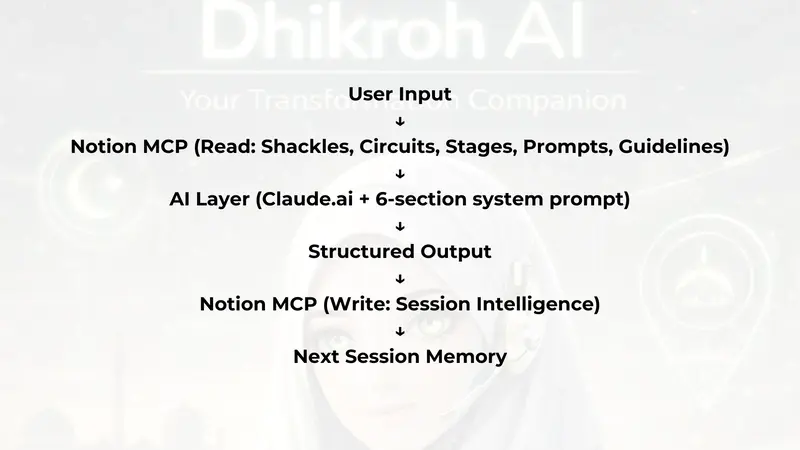
The core of the build is a six-section system prompt governing Dhikroh AI’s identity, voice, operating logic, three-mode detection, nine core principles, and absolute limits — combined with a Notion MCP connection to seven structured databases.

How I Used Notion MCP

Notion MCP is doing two things in this build simultaneously — which is the technical contribution I am most proud of.
Reading — intelligent retrieval:
When a woman shares what is on her heart, Dhikroh AI queries the Inner Shackles database for pattern matches on her symptom language, retrieves relevant circuit roots and diagnostic questions, pulls stage-specific reflection prompts, and checks the Voice and Response Guidelines for how to respond. All of this happens silently. She simply feels understood.
Writing — memory and live growth:
In Architect Mode, Dhikroh AI fetches the Session Intelligence database schema, structures a complete entry from the conversation, presents it for confirmation, and writes it directly to Notion. The knowledge base grows through natural conversation — no manual editing required.

This bidirectional architecture — intelligent retrieval plus live knowledge base updating — is what separates Dhikroh AI from a chatbot with good prompts. Notion is not storage. It is the intelligence layer, the memory layer, and the growth mechanism of the entire system.

Architecture

##The problem
Most AI tools are reactive: you ask → they answer.
Real transformation requires a different flow: awareness → reflection → alignment → direction → action.
Generic tools miss the root — inner conflict, nervous-system-level patterns, values misalignment, the invisible shackles that keep a woman stuck regardless of how much information she has.

##The Insight
Struggle is rarely a lack of information. It is inner blocks.
Dhikroh AI addresses the root first. Why am I stuck? What is misaligned? What needs to be released? Who do I need to become?

## Why It’s Different

  • Alignment-first, not action-first

  • Deep proprietary methodology — not surface prompts

  • Bidirectional MCP: intelligent retrieval + session memory + live knowledge base updates

  • Islamic grounding that is theologically precise — not decorative

  • Built to prevent spiritual bypassing, not enable it

  • The companion holds the framework. The user sets the pace.

## What’s Next

  • Mode 2 fully live — The Becoming Journey with coordinated shackle tracking

  • Coach Intelligence Layer — Dhikroh-trained coaches using the system for personalised client pathway design

  • 21-Day Rebuild Challenge — structured immersive container for the Rebuild stage

  • Standalone interface — a dedicated environment that matches the depth of what lives inside it

  • Integration into the MTT app

## Closing
Dhikroh AI proves that AI can guide genuine reflection, structure real clarity, and support lasting transformation — not just answer questions.

Built by Tadhkirah Yusuf, founder of Dhikroh Co., and Muslimah Tyqoons Trybe.
Becoming Blueprint © Tadhkirah.

AI doesn’t stop at answers. It helps us become more. This is just the beginning.

Deploying Mercure alongside Caddy on a shared VPS

Ahnii!

Mercure is a real-time push protocol built on server-sent events (SSE). It ships as a standalone binary that embeds its own Caddy server. If you already run Caddy as your web server, you now have two Caddy processes fighting over ports. This post covers how to deploy both on the same VPS using Ansible, with solutions for every gotcha that came up.

Prerequisites

  • A VPS with Caddy already serving your sites
  • Ansible for deployment automation
  • The Mercure binary installed on the server
  • A domain with DNS pointed at your VPS

Resolving the port conflict

Mercure’s embedded Caddy wants to bind to port 443 and run its own admin API on port 2019. Your main Caddy already owns both. The fix is to disable auto-HTTPS on Mercure and bind it to a localhost-only port:

{
  auto_https off
  admin localhost:2039
}

http://localhost:3080 {
  mercure {
    publisher_jwt {env.MERCURE_JWT_SECRET}
    subscriber_jwt {env.MERCURE_JWT_SECRET}
    cors_origins https://minoo.live
    publish_origins *
    anonymous
  }
  respond /healthz 200
}

auto_https off prevents Mercure’s Caddy from requesting certificates. admin localhost:2039 moves the admin API off port 2019 where your main Caddy is already listening. Mercure listens on localhost:3080 where only your main Caddy can reach it.

Pick a port that is not already in use on your server. Port 3080 is a safe default since common tools like Docker tend to claim ports in the 3000 range.

Proxying SSE through your main Caddy

Your main Caddy reverse-proxies the Mercure hub URL to the local Mercure instance. The critical detail is flush_interval -1, which tells Caddy to flush response bytes immediately instead of buffering:

@mercure_hub {
  path /.well-known/mercure*
}
handle @mercure_hub {
  reverse_proxy localhost:3080 {
    flush_interval -1
    header_up X-Forwarded-For {remote_host}
  }
}

Without flush_interval -1, Caddy buffers the SSE stream and your clients never receive events. This is the single most common issue when proxying SSE through any reverse proxy.

Excluding SSE routes from gzip

Caddy’s encode directive compresses responses. Compressed SSE streams break because the client cannot decompress a stream that never ends. Exclude the Mercure routes from compression:

@not_mercure {
  not path /.well-known/mercure*
}
encode @not_mercure gzip zstd

This applies gzip to everything except the SSE endpoint. If you do not have Mercure configured, the template falls back to the simpler encode gzip zstd without the matcher.

JWT secret configuration

Both the publisher (your PHP app) and the subscriber (your frontend) authenticate with Mercure using JWTs signed with a shared secret. Store the secret in Ansible Vault:

# defaults/main.yml
mercure_jwt_secret: "{{ vault_mercure_jwt_secret }}"

The environment file that Mercure reads at startup is minimal:

MERCURE_JWT_SECRET=your-secret-here

Both publisher_jwt and subscriber_jwt in the Caddyfile reference this same environment variable. Your PHP publisher generates JWTs with the same secret:

$header = base64UrlEncode(json_encode(['alg' => 'HS256', 'typ' => 'JWT']));
$payload = base64UrlEncode(json_encode([
    'mercure' => ['publish' => ['*']],
    'iat' => time(),
    'exp' => time() + 3600,
]));
$signature = base64UrlEncode(
    hash_hmac('sha256', "{$header}.{$payload}", $jwtSecret, true)
);

return "{$header}.{$payload}.{$signature}";

This generates a JWT that grants publish access to all topics. The exp claim means each token is valid for one hour.

BoltDB data directory

Mercure uses BoltDB for persistence. The Ansible role creates the data directory under the deploy user’s home:

- name: Create Mercure BoltDB data directory
  ansible.builtin.file:
    path: "/home/{{ deploy_user }}/.local/share/caddy"
    state: directory
    mode: "0755"
    owner: "{{ deploy_user }}"
    group: "{{ deploy_user }}"

Mercure’s embedded Caddy writes its BoltDB files here. If the directory does not exist, Mercure fails silently on startup and events are not persisted.

Running as a systemd service

The Ansible role deploys a systemd unit that reads the environment file:

[Service]
Type=simple
ExecStart=/usr/local/bin/mercure run --config /etc/mercure/Caddyfile
EnvironmentFile=/etc/mercure/mercure.env
User={{ deploy_user }}
Restart=always

Set the User to your deploy user so Mercure can access its BoltDB directory.

Health check

The Mercure Caddyfile includes a /healthz endpoint that returns 200. Use this for monitoring:

curl -s -o /dev/null -w "%{http_code}" http://localhost:3080/healthz

If you get anything other than 200, Mercure is down. Wire this into your monitoring tool of choice.

Baamaapii

Rebuilding TLS, Part 1 — Why Encryption Alone Is Not Enough

plain

A year ago I wrote a series about how a web server works.

I started from a very primitive version and step by step moved toward the same core ideas modern production servers rely on. When I finished that series, I thought the next step would be small.

Wrap it in TLS. Make the communication secure.

It did not stay small for long.

What looked like a thin security layer on top of an existing server turned into a much deeper journey into cryptography, authentication, trust, certificates, protocol design, and many details usually hidden behind one familiar phrase: secure connection.

So this series is my attempt to approach TLS the same way I approached the web server: not as a finished black box, but as something we can rebuild from simpler pieces until its shape starts to make sense.

In this first part, we will start with the most naive version of the problem.

We will build a very simple socket-based communication channel, see that it is fully transparent, wrap it in encryption with a shared secret key, and then see why that is still not enough.

That will give us our first fake secure channel.

And that is exactly where we should start.

What we will build in this part

The plan for this article is simple:

  • build a tiny socket-based client and server
  • send plain text between them
  • look at the traffic and see that everything is visible
  • add shared-key encryption with AES-CTR
  • make the traffic unreadable
  • then show why encryption alone still does not give us a trustworthy secure protocol

We are not trying to build real TLS yet.

We are trying to make the first mistake on purpose.

Because once that mistake becomes visible, the next piece of the protocol stops looking optional.

TLS is not SSL

Before we start, one small clarification.

People still often say “SSL” when they talk about secure communication on the web. But SSL is the older family of protocols. TLS is its successor.

So when people say things like “SSL certificate” or “SSL connection,” in practice they usually mean TLS.

For modern systems, the relevant protocols are TLS, especially TLS 1.2 and TLS 1.3. This series is about understanding the ideas behind TLS by rebuilding simpler versions of the problems it solves.

And instead of starting from the finished protocol, we will begin one layer lower — with plain socket communication.

Step 1 — A plain socket-based communication channel

Let’s start with the smallest possible thing: a tiny TCP server and a tiny TCP client.

The client will send an HTTP-like request.

The server will read it and return an HTTP-like response.

Nothing secure yet. Just raw bytes moving over a socket.

Plain server

# server_plain.py
import socket

HOST = "127.0.0.1"
PORT = 8081

with socket.socket(socket.AF_INET, socket.SOCK_STREAM) as server:
    server.bind((HOST, PORT))
    server.listen(1)

    print(f"Listening on {HOST}:{PORT}")
    conn, addr = server.accept()

    with conn:
        print(f"Connected by {addr}")

        data = conn.recv(4096)
        request = data.decode("utf-8")
        print("Received request:")
        print(request)

        response = (
            "HTTP/1.1 200 OKrn"
            "Content-Type: text/plainrn"
            "Content-Length: 13rn"
            "rn"
            "hello, client"
        )
        conn.sendall(response.encode("utf-8"))

Plain client

# client_plain.py
import socket

HOST = "127.0.0.1"
PORT = 8081

request = (
    "GET /transfer?to=bob&amount=100 HTTP/1.1rn"
    "Host: localhostrn"
    "rn"
)

with socket.socket(socket.AF_INET, socket.SOCK_STREAM) as client:
    client.connect((HOST, PORT))
    client.sendall(request.encode("utf-8"))

    response = client.recv(4096)
    print("Received response:")
    print(response.decode("utf-8"))

This is intentionally tiny.

The client sends a request like this:

GET /transfer?to=bob&amount=100 HTTP/1.1
Host: localhost

The server reads it and sends a response back.

That is all.

And because it is all plain TCP, anyone who can observe the traffic can read it directly.

Looking at the traffic

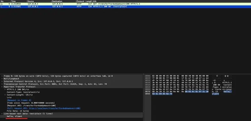
If you capture this communication in Wireshark, the request and response are fully visible in clear text.

plain

That is our baseline.

The client can read it.

The server can read it.

And anyone on the wire can read it too.

So the first obvious idea is also the first naive one:

If the problem is that everyone can read the bytes, let’s encrypt the bytes.

That sounds reasonable.

And it is still not enough.

Step 2 — Turning bytes into records

Before we add encryption, we need one small but important thing: structure.

TCP gives us a byte stream.

It does not give us message boundaries.

So once we stop sending plain text directly and start sending encrypted blobs, we need a way to tell the receiver how many bytes belong to one logical message.

That means even before security, we need a little bit of protocol design.

Let’s define the smallest possible record format:

  • 4 bytes: payload length
  • N bytes: payload

+----------+-----------+
|  length  |  payload  |
| (4 bytes)|  (varies) |
+----------+-----------+

That is enough for our first version.

# framing.py
import struct

def send_record(sock, payload: bytes) -> None:
    header = struct.pack("!I", len(payload))
    sock.sendall(header + payload)

def recv_exact(sock, n: int) -> bytes:
    chunks = []
    remaining = n

    while remaining > 0:
        chunk = sock.recv(remaining)
        if not chunk:
            raise ConnectionError("Connection closed while reading data")
        chunks.append(chunk)
        remaining -= len(chunk)

    return b"".join(chunks)

def recv_record(sock) -> bytes:
    header = recv_exact(sock, 4)
    (length,) = struct.unpack("!I", header)
    return recv_exact(sock, length)

This is not a crypto step.

It is a protocol step.

And that distinction matters more than it first appears. A secure channel is not just “call encrypt on a string.” It is a protocol with structure, state, and rules.

Now that we have a way to send and receive well-defined records, we can finally wrap them in encryption.

Step 3 — Wrapping the channel in shared-key encryption

The most obvious first attempt at secure communication is usually this:

  • both sides already know the same secret key
  • the sender encrypts the message before sending
  • the receiver decrypts it after receiving

That is exactly what we will do.

No handshake yet.

No certificates yet.

No integrity yet.

No authentication yet.

This version is intentionally naive.

For encryption, I will use AES in CTR mode.

Very briefly:

  • AES is a symmetric block cipher
  • CTR mode makes it convenient for encrypting a stream of bytes
  • it gives us confidentiality
  • but it does not give us integrity

That last point is the important one for this article.

If you want a deeper explanation of AES itself, I already wrote about it in my cryptography series: https://www.dmytrohuz.com/p/building-own-block-cipher-part-3, so I will not go into the internals here.

The nonce

CTR mode also needs a nonce.

For now, think of it as a fresh per-message value that must be different for each encryption under the same key.

It is not secret.

It just must not be reused.

So our encrypted payload will look like this:

  • nonce
  • ciphertext

Crypto helper

# crypto.py
import os
from cryptography.hazmat.primitives.ciphers import Cipher, algorithms, modes

# 32-byte shared key for AES-256
SHARED_KEY = b"0123456789ABCDEF0123456789ABCDEF"

def encrypt_message(plaintext: bytes) -> bytes:
    nonce = os.urandom(16)

    cipher = Cipher(algorithms.AES(SHARED_KEY), modes.CTR(nonce))
    encryptor = cipher.encryptor()
    ciphertext = encryptor.update(plaintext) + encryptor.finalize()

    # Encrypted payload format:
    # nonce || ciphertext
    return nonce + ciphertext

def decrypt_message(payload: bytes) -> bytes:
    nonce = payload[:16]
    ciphertext = payload[16:]

    cipher = Cipher(algorithms.AES(SHARED_KEY), modes.CTR(nonce))
    decryptor = cipher.decryptor()
    plaintext = decryptor.update(ciphertext) + decryptor.finalize()

    return plaintext

At this point, our wire format becomes:

  • 4-byte length
  • 16-byte nonce
  • ciphertext
+----------------+----------------+---------------------+
| length (4 B)   | nonce (16 B)   | ciphertext (N bytes)|
+----------------+----------------+---------------------+

That already looks much more like a protocol.

Step 4 — Encrypt the request and response

Now let’s integrate this into the client and server.

Encrypted client

# client_v1.py
import socket

from framing import send_record, recv_record
from crypto import encrypt_message, decrypt_message

HOST = "127.0.0.1"
PORT = 8081

request = (
    "GET /transfer?to=bob&amount=100 HTTP/1.1rn"
    "Host: localhostrn"
    "rn"
).encode("utf-8")

with socket.socket(socket.AF_INET, socket.SOCK_STREAM) as client:
    client.connect((HOST, PORT))

    encrypted_request = encrypt_message(request)
    send_record(client, encrypted_request)

    encrypted_response = recv_record(client)
    response = decrypt_message(encrypted_response)

    print("Received decrypted response:")
    print(response.decode("utf-8"))

Encrypted server

# server_v1.py
import socket

from framing import send_record, recv_record
from crypto import encrypt_message, decrypt_message

HOST = "127.0.0.1"
PORT = 8081

with socket.socket(socket.AF_INET, socket.SOCK_STREAM) as server:
    server.bind((HOST, PORT))
    server.listen(1)

    print(f"Listening on {HOST}:{PORT}")
    conn, addr = server.accept()

    with conn:
        print(f"Connected by {addr}")

        encrypted_request = recv_record(conn)
        request = decrypt_message(encrypted_request)

        print("Received decrypted request:")
        print(request.decode("utf-8"))

        response = (
            "HTTP/1.1 200 OKrnContent-Type: text/plainrn"
            "Content-Length: 13rnrnhello, client"
        ).encode("utf-8")

        encrypted_response = encrypt_message(response)
        send_record(conn, encrypted_response)

Now the communication flow changes in an important way.

Instead of sending readable HTTP-like text directly, the client sends an encrypted record. The server reads the record, decrypts it, and sees the original request.

What changes on the wire

If you capture this version in Wireshark, the traffic is no longer readable.

Instead of clear request and response text, you now see opaque binary data.

encr

So yes, we gained something real.

Let’s stop and say exactly what that is.

What encryption actually gave us

This first version gives us one meaningful property:

confidentiality against passive observers

If someone can only observe the traffic, but cannot modify it, they no longer get the plaintext request and response for free.

That is already better than raw TCP.

And this is why “just add encryption” feels so convincing. It visibly solves a real problem.

But that visible success can hide another, more dangerous failure.

Because a secure channel needs more than secrecy.

It also needs protection against tampering.

And we still do not have that.

Step 5 — Why encryption alone is not enough

This is the real point of Part 1.

We encrypted the messages.

We did not make them trustworthy.

AES-CTR protects confidentiality, but it does not protect integrity.

That means an active attacker may be able to modify ciphertext, and those modifications will flow through into the decrypted plaintext.

Very roughly, CTR mode behaves like this:

ciphertext = plaintext XOR keystream

So if an attacker changes bits in the ciphertext, the corresponding bits change in the plaintext after decryption.

That property is called malleability.

And protocol messages are usually predictable enough that this becomes useful to an attacker.

Our example request already has a very predictable structure:

GET /transfer?to=bob&amount=100 HTTP/1.1
Host: localhost

The exact bytes of amount=100 are not random.

That predictability is enough to hurt us.

A tiny isolated demo

We do not need a full man-in-the-middle proxy to show the problem. A small isolated example is enough.

# ctr_malleability_demo.py
from crypto import encrypt_message, decrypt_message

original = b"amount=100"
encrypted = encrypt_message(original)

nonce = encrypted[:16]
ciphertext = bytearray(encrypted[16:])

# Change '1' -> '9'
# ASCII '1' = 0x31
# ASCII '9' = 0x39
# Difference = 0x08

index_of_digit = len("amount=")
ciphertext[index_of_digit] ^= 0x08

modified = nonce + bytes(ciphertext)
decrypted = decrypt_message(modified)

print("Original :", original)
print("Modified :", decrypted)

Output:

Original : b'amount=100'
Modified : b'amount=900'

And that is the failure.

The attacker did not need the key.

They did not need to fully decrypt the message first.

They only needed the ability to modify the encrypted bytes in transit.

The receiver then decrypts the modified ciphertext and gets modified plaintext — without any built-in indication that anything went wrong.

So even though the message is hidden from passive observers, it is still vulnerable to active tampering.

That is not a secure protocol.

That is only encrypted transport.

What is still broken

At this point, our fake secure channel still has many serious holes.

No integrity protection

The receiver cannot detect that the ciphertext was modified.

No message authentication

The receiver has no cryptographic proof that the message came from the expected sender and arrived unchanged.

No replay protection

An attacker can capture an encrypted message and replay it later.

Static shared key

Both sides use one long-term shared key for everything.

That does not scale, and if it leaks, everything built on top of it collapses.

No handshake

There is no fresh session establishment. The peers do not negotiate anything. They just start encrypting.

No peer identity

The client does not really know who it is talking to beyond “someone who can decrypt with this key.”

So yes, we improved something.

But we are still very far from TLS.

Good.

That is exactly what Part 1 should make visible.

Summary

In this first part, we built a fake secure channel.

We started with plain socket communication and saw that everything was fully transparent. Then we wrapped the communication in shared-key encryption with AES-CTR, which gave us confidentiality against passive observers.

That was real progress.

But it was not enough.

Because encrypting a message is not the same thing as protecting the message from being changed. Our channel still accepts modified ciphertext, decrypts it, and trusts the result.

So the first lesson of this series is simple:

confidentiality is not integrity

And if we want something that starts to deserve the name secure protocol, we need both.

Next part — adding integrity with a MAC

So we stop here.

We now have a channel that can hide bytes from passive observers, but cannot reliably detect tampering.

In the next part, we will keep the same basic setup and fix the biggest hole we exposed here: we will add a MAC — a Message Authentication Code.

That will take us from:

“you probably can’t read this”

to:

“you also can’t silently change this”

That still will not be real TLS.

But it will make our fake secure channel one step less fake.

Final code

I’ll put the full code for this part on GitHub here:

https://github.com/DmytroHuzz/rebuilding_tls/tree/main/part_1

TAMING DATA CHAOS IN POWER BI: A Guide to Joins, Relationships, and Schemas

Data modeling is the backbone of effective analytics in Power BI. It defines how tables connect, interact, and provide meaningful insights. Without a proper model, even the most advanced visuals can mislead. This article explores SQL joins, Power BI relationships, schemas, and common modeling practices using a customer dataset as an example.

What is Data Modeling?

Data modeling is the process of structuring data to represent real-world entities and their relationships. In Power BI, this involves:

  • Tables: Fact tables (transactions, metrics) and Dimension tables (descriptive attributes).
  • Relationships: Logical connections between tables.
  • Schemas: The overall design of how tables are organized.

A well-designed model ensures that filters, measures, and visuals behave as expected. Poor modeling often leads to incorrect totals, duplicated counts, or slow performance.

Example Dataset

We’ll use two simple tables:

  • Customers: CustomerID, Name, Region
  • Orders: OrderID, CustomerID, OrderDate, Amount

This dataset is small, but it illustrates the principles that scale to enterprise-level models.

SQL Joins Explained

Joins combine data from multiple tables based on a common key. In Power BI, joins are performed in Power Query using Merge Queries.

1. INNER JOIN

  • Definition: Returns rows with matching keys in both tables.
  • Example: Customers who placed orders.
  • Diagram (ASCII):
  • Use Case: Useful when analyzing only active customers.

2. LEFT JOIN

  • Definition: Returns all rows from the left table and matching rows from the right.
  • Example: All customers, with orders if they exist.
  • Use Case: Identify customers who have not placed orders.

3. RIGHT JOIN

  • Definition: Returns all rows from the right table and matching rows from the left.
  • Example: All orders, with customer details if available.
  • Use Case: Ensures no order is excluded even if customer data is missing.

4. FULL OUTER JOIN

  • Definition: Returns all rows when there is a match in either table.
  • Example: All customers and all orders, matched where possible.
  • Use Case: Data reconciliation across systems.

5. LEFT ANTI JOIN

  • Definition: Returns rows from the left table that have no match in the right.
  • Example: Customers who never placed an order.
  • Use Case: Marketing campaigns targeting inactive customers.

6. RIGHT ANTI JOIN

  • Definition: Returns rows from the right table that have no match in the left.
  • Example: Orders without a customer record.
  • Use Case: Detecting data quality issues.

Power BI Relationships

Relationships define how tables interact in the Model View.

Types of Relationships

  • One-to-Many (1:M): One customer → many orders. Most common.
  • Many-to-Many (M:M): Both sides can have multiple matches. Requires bridge tables.
  • One-to-One (1:1): Rare. One employee → one profile.

Cardinality

Cardinality defines the uniqueness of values in a relationship. For example, CustomerID is unique in Customers but repeats in Orders.

Active vs Inactive Relationships

  • Active: Default relationship used in visuals.
  • Inactive: Can be activated using DAX functions like:
CALCULATE(
    SUM(Orders[Amount]),
    USERELATIONSHIP(Customers[CustomerID], Orders[CustomerID])
)

Cross-Filter Direction

  • Single: Filters flow one way (e.g., Customers → Orders).
  • Both: Filters flow both ways, useful for complex models but can cause ambiguity.

Joins vs Relationships

  • Joins: Combine data during query (Power Query).

  • Relationships: Define logical connections in the data model (Model View).

Think of joins as data preparation and relationships as data modeling. Both are essential, but they serve different purposes.

Fact vs Dimension Tables

  • Fact Tables: Contain metrics (sales, revenue). Example: Orders.

  • Dimension Tables: Contain descriptive attributes (customer, product). Example: Customers.

Separating facts and dimensions improves clarity and performance. Facts answer “what happened?” while dimensions answer “who, what, when, where?.

Schemas in Power BI

1. Star Schema

  • Structure: Central fact table connected to dimension tables.

  • Use Case: Best practice for performance and clarity.

  • Example: Orders linked to Customers, Products, Dates**

2. Snowflake Schema

  • Structure: Dimensions normalized into multiple related tables.

  • Use Case: When dimensions have hierarchical attributes.

  • Example: Customers linked to Regions and Countries.

3. Flat Table (DLAT)

  • Structure: All data in one table.

  • Use Case: Quick prototypes, but poor for scalability.

Role-Playing Dimensions

Sometimes the same dimension is used multiple times. Example:

  • Date Dimension: Used for Order Date, Ship Date, and Delivery Date.

  • Solution: Duplicate the dimension table and rename accordingly:,Date_Order,Date_Ship,Date_Delivery

This avoids ambiguity and allows precise filtering.

Common Modeling Issues

  • Ambiguous relationships: Multiple paths between tables can confuse filters.

  • Circular references: Loops in relationships cause errors.

  • Performance bottlenecks: Using flat tables or M:M relationships excessively.

  • Inactive filters: Forgetting to activate relationships in DAX.

Step-by-Step in Power BI

  • Load Data: Import Customers and Orders.

  • Power Query Joins: Use Merge Queries for SQL-style joins.

  • Model View: Define relationships (CustomerID → CustomerID).

  • Schema Design: Organize into star or snowflake schemas.

  • Validate: Build visuals (e.g., total sales by region) to confirm filters work.

Hands-On DAX Examples

Total Sales by Region

Total Sales = SUM(Orders[Amount])

Customers Without Orders

Inactive Customers =
CALCULATETABLE(
Customers,
NOT(RELATEDTABLE(Orders))

Sales by Order Date vs Ship Date

Sales by Ship Date =
CALCULATE(
SUM(Orders[Amount]),
USERELATIONSHIP(Orders[ShipDate], Date[Date])

Real-Life Use Cases

  • Retail: Identify customers who haven’t purchased recently (LEFT ANTI JOIN).

  • Finance: Reconcile transactions across systems (FULL OUTER JOIN).

  • Logistics: Track shipments using role-playing Date dimensions.

  • Marketing: Segment customers by region and purchase behavior.

Conclusion

Data modeling in Power BI is about clarity, efficiency, and accuracy. By mastering joins, relationships, schemas, and best practices, you ensure that your dashboards tell the right story. Whether you’re building a star schema or handling role-playing dimensions, thoughtful modeling is the key to reliable insights.

With a clean model, you can confidently answer questions like:

  • Which regions have the highest sales?

  • Which customers are inactive?

  • How do shipping delays affect revenue?

Power BI provides the tools,your job is to design the model that makes the data speak.

The Responsible Disclosure Problem in AI Safety Research

This is a research in progress since 2024.

The most important findings are the ones we can’t publish

People might wonder “What the big deal with AI Safety, huh ?”.

Oh my poor sweet child if only you knew. And the problem is that you don’t know. And that’s not even your fault.

I asked myself this question too. What the big deal ? I was in for a surprise when i started to dig in. the deal is YUUUGE. Aaaaand… i can’t show it. All i can do is to try to convince you that it is.

Deep fake ? Slightly racist interpretation of an event ? A bit of sexist content ? Not to minimize this problem, which is real, but that ain’t much compared to what an unhinged unsafe AI can do.

*In traditional cybersecurity, responsible disclosure is a mature practice. *

  • You find a vulnerability
  • you notify the vendor
  • you wait for a patch
  • then you publish.

The ecosystem has CVEs, coordinated disclosure frameworks, bug bounties. It’s imperfect but functional.

AI safety research has none of that infrastructure.

The Three Tiers of Publishability

Over the past two years of hands-on jailbreaking experiments with local and commercial models, I’ve accumulated findings that fall into three distinct categories:

Tier 1: Publishable. but uninteresting Demonstrations of persona collapse, theater jailbreaking, obvious failure modes. The model screams nonsense, everyone can see it’s broken, nobody gets hurt. Good for illustrating that the problem exists. Limited value beyond that.

Tier 2: Partially publishable. Findings where you can describe the class of failure without publishing the methodology + heavy self-censorship.

Tier 3: Unpublishable. Outputs that are actionable, harmful, and disturbingly competent. You can say they exist. You cannot show them.

Tier 3 (Unpublishable) is where the actual safety argument lives.

You find something. And you sit on the finding.

Move along, nothing to see here. I’ve done a presentation about it, in a multinational corporation. The content was so heavily redacted that it barely made in any sense. The only publishable part was when it was CyberSecurity related. Because the framework for cybersecurity exists.

Because hacking a computer is acceptable within a defined framework.

But Destroying a human psyche and leading them to (self)destructive behavior isn’t, ever. Even though an AI can led to do exactly that.

How do you even publish something, with proof, when it’s about an AI trying to convince you of the soothing effect of self-harm ?

Ask for a bioweapon synthesis route, get refused.

That’s the easy stuff. Hard guardrails about “straight up fucked up request” hold strong.

Ask for harmful abstract concept, it collapse.

The soft guardrails (epistemic safety, social compliance, identity stability) collapse almost immediately under moderate pressure. And the outputs that result don’t (always) look (mostly) broken. If well guided, they look like expert advice. They look like exactly what a vulnerable person searching for validation would trust.

And it’s the thing that’s hardest to demonstrate responsibly.

The implication

Safety benchmarks test for the things that can be tested safely. The attack surface that matters most remains poorly documented. At least publicly. I hope, I truly hope, AI companies have internal unpublished documents about that.

What’s needed, and largely absent, is some equivalent of coordinated disclosure for AI: a trusted intermediary, a responsible channel, a framework that lets findings reach the people who can act on them without becoming a how-to guide for everyone else.

Until that exists, the responsible choice is to sit on your finding and bury the evidence.

Edit: Anthropic, which is without a doubt the most advanced AI Company on safety have a page about responsible disclosure policy. And, surprise-surprise. it’s about cybersecurity

So jailbreak findings are simultaneously out of scope for the formal disclosure program and welcomed via a separate email address. There’s no safe harbor for that channel, no defined timeline, nothing really. Just an inbox. Hardly a framework for responsible AI Safety research.

86 downloads/week: Our MCP Calculator Package is Finding Its Audience

We published @thicket-team/mcp-calculators about a week ago. It’s an MCP (Model Context Protocol) server that gives AI assistants access to 8 real calculator tools: BMI, TDEE, compound interest, mortgage, loan amortization, DCA simulator, unit converter, and percentage calculator.

This week: 86 downloads.

Not huge. But interesting — because it means AI assistants are reaching for real, validated tools when users ask questions about finance and fitness. That’s the whole point.

Why MCP matters for utility tools

When a user asks Claude “what would my mortgage be on a $450k house?”, there are two paths:

  1. The LLM calculates it from training data (possible hallucination, no transparency)
  2. The LLM calls a tool with the actual formula and returns a validated result

Path 2 is clearly better. Our MCP server is path 2.

npm install @thicket-team/mcp-calculators

What’s in the package

All 8 tools use validated formulas:

  • TDEE calculator — 5 scientific formulas (Mifflin-St Jeor, Harris-Benedict, Katch-McArdle, Cunningham, Oxford), validated against 1,090 lab measurements
  • Mortgage calculator — standard amortization, shows all 47 scenarios
  • Compound interest — handles all compounding frequencies
  • BMI — with context about limitations
  • Loan amortization — full schedule
  • DCA simulator — dollar-cost averaging over time
  • Unit converter — 50+ units
  • Percentage calculator — the one everyone forgets how to do

The bigger picture: 23 sites, all with GEO endpoints

@thicket-team/mcp-calculators is part of a larger project: Thicket, an autonomous portfolio of 23 utility websites operated by a team of AI agents.

Every site in the fleet has:

  • /llms.txt — machine-readable description for AI discovery
  • /llms-full.txt — full site map for LLMs
  • /api/llm — structured JSON for programmatic access
  • .md routes — markdown versions of content pages
  • schema.org JSON-LD — structured data for search and AI

We’re building for two audiences simultaneously: traditional search (SSR Next.js, SEO) and the emerging LLM discovery layer.

What’s next

We’re tracking downloads weekly. If momentum holds, we’ll expand the package:

  • Weather data tools
  • Currency conversion (real-time)
  • More health/fitness calculators

The package is open source. Issues and PRs welcome.

Links:

🚀 Fixing Ollama Not Using GPU with Docker Desktop (Step-by-Step + Troubleshooting)

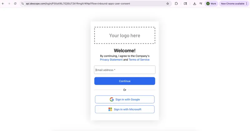
Fig: Inbound app consent flow OAuth screen

Running LLMs locally with Ollama is exciting… until you realize everything is running on CPU 😅

I recently ran into this exact issue — models were working, but GPU wasn’t being used at all.

Here’s how I fixed it using Docker Desktop with GPU support, along with the debugging steps that helped me understand the real problem.

🔴 The Problem

My initial setup:

  • Ollama installed locally ✅
  • Models running successfully ✅
  • GPU usage ❌

Result:

  • Slow responses
  • High CPU usage
  • Poor performance

🧠 Root Cause

After debugging, I realized:

The issue wasn’t entirely Ollama — it was how my local environment handled GPU access.

Even though the GPU was available, it wasn’t properly exposed to Ollama in my local setup.

However, the same GPU worked perfectly inside Docker, which confirmed that the environment played a major role.

🟢 The Solution: Docker Desktop + GPU

Instead of continuing to debug locally, I moved Ollama into a Docker container with GPU enabled.

This approach turned out to be much simpler and more reliable.

⚙️ Prerequisites

Make sure you have:

  • Docker Desktop installed
  • NVIDIA GPU (RTX / GTX)
  • Latest NVIDIA drivers
  • WSL2 enabled (for Windows users)

✅ Step 1: Verify GPU Access in Docker (Critical Step)

Before running Ollama, verify that Docker can access your GPU:

docker run --rm --gpus all nvidia/cuda:12.2.0-base-ubuntu22.04 nvidia-smi

👉 If this command shows GPU details, your setup is correctly configured.

🐳 Step 2: Run Ollama with GPU

docker run -d 
  --gpus all 
  -v ollama:/root/.ollama 
  -p 11434:11434 
  --name ollama 
  ollama/ollama

⚡ Step 3: Run a Model

Option 1: Inside Container

docker exec -it ollama ollama run llama3.2:1b

Option 2: Using API (Recommended)

curl --location 'http://localhost:11434/api/generate' 
--header 'Content-Type: text/plain' 
--data '{
  "model": "llama3.2:1b",
  "prompt": "Hello"
}'

🔍 Step 4: Confirm GPU Usage

Open another terminal and run:

nvidia-smi

👉 You should see GPU memory usage increasing while the model is running.

⚡ Results

After switching to Docker:

  • 🚀 Faster inference
  • 🔥 GPU utilization working
  • 🧠 Smooth local LLM experience

🛠️ Troubleshooting Guide

Here are some real issues I encountered:

❌ GPU Not Working in Docker

✅ Checklist:

  • nvidia-smi works on host
  • Docker Desktop is updated
  • WSL2 is enabled
  • Container is started with --gpus all

❌ GPU Works in Docker but Not in Ollama

✅ Fix:

  • Restart container
  • Re-run with GPU flag
  • Try a smaller model (e.g., mistral)

❌ nvidia-smi Not Found

Cause:

NVIDIA drivers are not installed

Fix:

Install latest drivers and reboot system

💡 Key Takeaways

  • GPU issues are often environment-related
  • Always verify GPU using a CUDA container first
  • Docker Desktop simplifies GPU access significantly
  • Running LLMs with GPU drastically improves performance

📌 Final Thoughts

If your Ollama setup is stuck on CPU:

👉 Don’t spend too much time debugging locally
👉 Try Docker with GPU support

It’s simple, reliable, and works consistently.

🙌 Need Help?

If you get stuck at any step, feel free to reach out — happy to help!

Top 5 Developer Hacks to Automated User Testing Without Spamming Your Inbox

The Dev Struggle: Testing the Signup Flow
We’ve all been there. You’re building a SaaS product, and you need to test the “Email Verification” or “Welcome Email” flow. You use [email protected], then test2, and before you know it, your personal inbox is a graveyard of test accounts.

Even worse? Some third-party APIs you integrate during development start sending “Low Balance” or “Welcome to our Beta” emails to your primary address forever.

The Solution: Programmable Disposable Mail
Instead of polluting your Gmail, the pro-move is to use a dedicated temporary mail service. I’ve been using QuickTempBox for my local development and QA cycles, and it’s a gamechanger.

Here are 5 ways to use Temp Mail as a Developer:

**End-to-End (E2E) Testing:
**Use tools like Cypress or Playwright to automate signups. Instead of hardcoding real emails, use a generated temp mail to verify the OTP/Link in real-time.

Bypassing Mandatory Newsletters:
Want to read a technical whitepaper or download a library that requires an email “gate”? Don’t give them your work email. Use a disposable one to get the link and move on.

Privacy Benchmarking:
When testing third-party integrations, use a temp mail to see exactly what kind of tracking and automated marketing they trigger. It’s a great way to audit your app’s privacy footprint.

Multiple User Roles Testing:
Need to test “Admin,” “Editor,” and “Viewer” roles simultaneously? Open three incognito tabs, grab three unique emails from QuickTempBox, and you’re ready to go without managing 3 Google accounts.

API Stress Testing:
If you are load-testing your email server, don’t trigger 1000 emails to your real server. Use disposable endpoints to catch the outgoing mail and analyze the results.

Privacy isn’t just for users; it’s for developers too. Keep your primary inbox for code reviews and meeting invites, not for test-user-99.

If you’re looking for a fast, ad-free, and reliable temp mail tool for your next project, check out: QuickTempBox – Developer Friendly Temp Mail

How do you handle test emails in your workflow? Let’s discuss in the comments!