Gas-Aware Trading: Execute Only When Gas Is Cheap

Your trading bot spotted a perfect arbitrage opportunity between Uniswap and Balancer. The price difference is 2.5% — enough for solid profit. But gas is sitting at 80 gwei. By the time the transaction confirms, the opportunity vanishes and you’re left holding the gas bill.

This scenario plays out thousands of times daily in DeFi. Trading bots either miss opportunities waiting for cheap gas or burn through profits on expensive transactions. What if your bot could automatically execute trades only when gas prices meet your profitability threshold?

Why Gas-Aware Execution Matters for Trading Bots

Gas costs can make or break trading strategies. A profitable arbitrage at 20 gwei becomes a loss at 100 gwei. MEV bots competing for the same opportunities often end up in gas wars, driving costs through the roof. Manual gas monitoring doesn’t scale when you’re running strategies across multiple chains and protocols.

The challenge isn’t just gas prices — it’s coordination. Your bot needs to:

  • Monitor gas prices across networks in real-time
  • Queue transactions with conditional execution
  • Cancel outdated opportunities before they become losses
  • Maintain execution across 14 DeFi protocols simultaneously
  • Handle cross-chain arbitrage where timing matters

Building this infrastructure from scratch means maintaining gas price feeds, transaction queuing systems, and integrations with dozens of protocols. That’s months of development before you even start on your actual trading logic.

Gas Conditional Execution: Your Bot Trades Smarter

WAIaaS solves this with gas conditional execution built into its 7-stage transaction pipeline. Your bot submits trades with gas price thresholds, and the system automatically executes only when conditions are met.

Here’s how it works in practice. Your arbitrage bot spots an opportunity and submits a conditional trade:

curl -X POST http://127.0.0.1:3100/v1/actions/jupiter-swap/swap 
  -H "Content-Type: application/json" 
  -H "Authorization: Bearer wai_sess_<token>" 
  -d '{
    "inputMint": "So11111111111111111111111111111111111111112",
    "outputMint": "EPjFWdd5AufqSSqeM2qN1xzybapC8G4wEGGkZwyTDt1v",
    "amount": "1000000000",
    "gasCondition": {
      "maxGasPrice": "50000000",
      "timeout": 300
    }
  }'

The transaction enters the pipeline and waits at stage 4 (wait) until gas drops below 50 lamports. If gas stays high for 300 seconds, the transaction expires automatically. No manual cancellation, no wasted gas on unprofitable trades.

Multi-Protocol Trading Through One API

Trading bots need access to liquidity across protocols. WAIaaS integrates 14 DeFi protocols through a unified API, so your bot can execute complex strategies without managing separate SDKs.

Execute a cross-protocol arbitrage in three API calls:

# 1. Swap on Jupiter (Solana)
curl -X POST http://127.0.0.1:3100/v1/actions/jupiter-swap/swap 
  -H "Authorization: Bearer wai_sess_<token>" 
  -d '{"inputMint": "SOL", "outputMint": "USDC", "amount": "10000000000"}'

# 2. Bridge to Ethereum via LI.FI
curl -X POST http://127.0.0.1:3100/v1/actions/lifi/bridge 
  -H "Authorization: Bearer wai_sess_<token>" 
  -d '{"fromChain": "solana", "toChain": "ethereum", "token": "USDC", "amount": "1000"}'

# 3. Lend on Aave v3
curl -X POST http://127.0.0.1:3100/v1/actions/aave-v3/supply 
  -H "Authorization: Bearer wai_sess_<token>" 
  -d '{"asset": "USDC", "amount": "1000"}'

Each action goes through the same gas-aware pipeline. Your bot submits the strategy, and WAIaaS handles execution timing across all three protocols.

Risk Controls That Scale

Trading bots need guardrails to prevent runaway losses. WAIaaS provides a 21-policy risk management system that operates at the wallet level, not per-strategy.

Set up automatic risk limits:

curl -X POST http://127.0.0.1:3100/v1/policies 
  -H "Content-Type: application/json" 
  -H "X-Master-Password: my-secret-password" 
  -d '{
    "walletId": "<wallet-uuid>",
    "type": "SPENDING_LIMIT",
    "rules": {
      "instant_max_usd": 1000,
      "notify_max_usd": 5000,
      "delay_max_usd": 20000,
      "delay_seconds": 300,
      "daily_limit_usd": 50000
    }
  }'

Trades under $1000 execute instantly. Trades between $1000-$5000 send notifications but still execute. Trades between $5000-$20000 wait 5 minutes (cancellable if your bot detects the opportunity expired). Trades over $20000 require manual approval.

You can also restrict protocols, tokens, and trading venues:

# Only allow trading on whitelisted protocols
curl -X POST http://127.0.0.1:3100/v1/policies 
  -H "X-Master-Password: my-secret-password" 
  -d '{
    "type": "CONTRACT_WHITELIST",
    "rules": {
      "contracts": [
        {"address": "JUP6LkbZbjS1jKKwapdHNy74zcZ3tLUZoi5QNyVTaV4", "name": "Jupiter"},
        {"address": "0x7d2768dE32b0b80b7a3454c06BdAc94A69DDc7A9", "name": "Aave"}
      ]
    }
  }'

Simulation and Backtesting

Before risking capital, test strategies with the dry-run API. Submit any transaction with "dryRun": true to see exactly what would happen:

curl -X POST http://127.0.0.1:3100/v1/transactions/send 
  -H "Content-Type: application/json" 
  -H "Authorization: Bearer wai_sess_<token>" 
  -d '{
    "type": "TRANSFER",
    "to": "recipient-address",
    "amount": "0.1",
    "dryRun": true
  }'

The response shows gas estimates, policy decisions, and potential errors without executing the transaction. Essential for backtesting strategies against historical gas prices.

High-Performance Bot Integration

Trading bots need minimal latency overhead. WAIaaS provides both REST APIs and TypeScript/Python SDKs optimized for high-frequency strategies:

import { WAIaaSClient } from '@waiaas/sdk';

const client = new WAIaaSClient({
  baseUrl: 'http://127.0.0.1:3100',
  sessionToken: process.env.WAIAAS_SESSION_TOKEN,
});

// Check opportunity profitability
const balance = await client.getBalance();
const gasPrice = await client.getGasPrice();

if (gasPrice < profitabilityThreshold) {
  // Execute arbitrage
  const tx = await client.executeAction('jupiter-swap', {
    inputMint: 'SOL',
    outputMint: 'USDC',
    amount: balance.balance
  });
}

The SDK handles connection pooling, request retries, and error handling so your bot focuses on trading logic, not infrastructure.

Quick Start: Gas-Aware Trading Bot

Get started with gas conditional execution in 5 steps:

  1. Deploy WAIaaS daemon:
git clone https://github.com/minhoyoo-iotrust/WAIaaS.git
cd WAIaaS
docker compose up -d
  1. Create a trading wallet:
npm install -g @waiaas/cli
waiaas quickset --mode mainnet
  1. Set up risk policies (spending limits, protocol whitelist, gas thresholds)

  2. Install the SDK:

npm install @waiaas/sdk
  1. Submit your first gas-conditional trade using the Jupiter swap example above

Your bot now executes trades only when gas conditions are favorable, with automatic risk controls and multi-protocol access.

What’s Next

This is just the beginning. WAIaaS supports perpetual futures on Hyperliquid, prediction markets on Polymarket, liquid staking, cross-chain bridging, and more. Each protocol integration includes gas-aware execution and risk controls out of the box.

Ready to build smarter trading bots? Check out the full documentation and examples at https://github.com/minhoyoo-iotrust/WAIaaS or visit https://waiaas.ai to get started.

Reflective — AI journaling companion built with Notion MCP and Claude

This is a submission for the Notion MCP Challenge

What I Built

Reflective is a Chrome extension + Node.js backend that adds an AI journaling companion to your browser sidebar while you write in Notion.

Most journaling tools are write-only. You pour thoughts in, they sit there. Reflective makes your Notion journal a two-way conversation — without leaving the page.

How it works:

You write in Notion
       ↓
Click "Analyze this entry" in the sidebar
       ↓
Claude reads your entry + your journal history from Notion
       ↓
Opens a conversation grounded in what you actually wrote
       ↓
Click "Mark session complete"
       ↓
Mood score, tags, themes, and AI summary written back to Notion

Key behaviors:

  • Sits in the Chrome side panel alongside Notion — no new tabs
  • Context-aware: on a database view it loads your last 50 entries; on a single entry it reads just that page
  • Temporal awareness: if you’re reading an old entry, Claude knows — it frames responses as looking back, not as if it’s today
  • One conversation across the whole session — navigating to a new entry appends to the chat with a — now reading: [title] — divider
  • Analysis is always user-initiated. The extension makes zero API calls on navigation.
  • Mood sparkline shows your last 14 days, pulled live from a Notion database

One-click workspace setup. On first launch, it creates a Journal Entries database, Mood Log, Weekly Summaries database, a seeded starter entry, and a dashboard page — all via the Notion API. You paste your integration token, it does the rest in ~10 seconds.

Video Demo

Show Us the Code

Repo: https://github.com/neicore/notion-reflective

Stack:

  • Chrome Extension (Manifest V3, React + TypeScript, Vite, Tailwind)
  • Node.js + Express backend (TypeScript)
  • Anthropic Claude (claude-sonnet-4-5)
  • Notion API (@notionhq/client v2)
  • Server-Sent Events for streaming progress to the extension
  • pnpm workspaces

How I Used Notion MCP

Notion is where users read and write their data — and it’s also the entire data model. Every piece of state lives there, accessed via @notionhq/client.

Reading: building context for Claude

When you click “Analyze this entry”, the backend fetches in parallel:

const [rawHistory, recentMoods] = await Promise.all([
  fetchJournalEntries(journalDbId, 50, notionToken),  // last 50 entries
  queryMoodHistory(moodLogDbId, 14, notionToken),      // 14-day sparkline
])

Then reads the current page blocks directly:

const [pageObj, blocks] = await Promise.all([
  notion.pages.retrieve({ page_id: pageId }),
  notion.blocks.children.list({ block_id: pageId, page_size: 100 }),
])

The block content becomes the raw text fed to Claude alongside journal history. History is split into “before this date” and “after this date” relative to the entry you’re viewing — that’s what gives Claude correct temporal framing.

Writing: analysis flows back into Notion

When you mark a session complete:

await notion.pages.update({
  page_id: pageId,
  properties: {
    'Mood Score':       { number: result.moodScore },
    'Mood Tags':        { multi_select: result.moodTags.map(name => ({ name })) },
    'Themes':           { multi_select: result.themes.map(name => ({ name })) },
    'AI Summary':       { rich_text: [{ text: { content: result.aiSummary } }] },
    'Word Count':       { number: wordCount },
    'Session Complete': { checkbox: true },
  },
})

Your Notion database gets richer over time. On future analyses, entries with an AI Summary are used as-is (fast); entries without one get their blocks fetched (slower, shown in the loading progress bar). First load hydrates your journal — subsequent loads are instant.

The loading experience

Hydrating 50 entries takes a while the first time. The /api/init endpoint streams progress via Server-Sent Events:

data: {"type":"journal_count","total":47}
data: {"type":"hydrating","index":1,"total":47,"title":"March reflections"}
data: {"type":"hydrating","index":2,"total":47,"title":"A hard week"}
...
data: {"type":"done","entryContent":"...","openingMessage":"..."}

The extension consumes this with fetch + ReadableStream (more reliable than EventSource in extension contexts), updating the UI: Reading your journal — 3/47 — A hard week.

What Notion unlocks that a plain database wouldn’t

Notion’s multi-select properties for Mood Tags and Themes mean once entries are analyzed, you can filter, sort, and group your entire journal by mood or theme natively in Notion — no custom query interface needed. The AI populates the properties; Notion’s built-in views do the rest.

The mood sparkline pulls from a separate Mood Log database that tracks daily mood independently from journal entries. You can log mood on days you don’t write, and the chart reflects it. Two related databases — the kind of structure that’s natural in Notion and would need real schema design anywhere else.

That’s the part I keep coming back to: the AI populates the properties, Notion’s built-in views do the rest. No custom query interface, no separate dashboard to maintain. Your journal just gets smarter over time.

Fresh 2 Has a Free API That Brings Zero-JS Pages to Deno With Island Architecture

Fresh is Deno’s web framework. Zero JavaScript shipped to the client by default. Interactive parts are “islands” that hydrate independently. Fresh 2 adds Preact Signals, better plugins, and faster builds.

Quick Start

deno run -A https://fresh.deno.dev my-app
cd my-app && deno task start

Zero JS by Default

Every Fresh page is server-rendered HTML. No JavaScript bundle. This page component ships 0 bytes of JS:

// routes/index.tsx
export default function Home() {
  return (
    <div>
      <h1>Hello Fresh</h1>
      <p>This page has zero client-side JavaScript.</p>
    </div>
  )
}

Islands (Interactive Components)

Only components in /islands/ get hydrated on the client:

// islands/Counter.tsx
import { useSignal } from "@preact/signals"

export default function Counter() {
  const count = useSignal(0)
  return (
    <div>
      <p>Count: {count}</p>
      <button onClick={() => count.value++}>+1</button>
    </div>
  )
}
// routes/index.tsx
import Counter from "../islands/Counter.tsx"

export default function Home() {
  return (
    <div>
      <h1>Static content (0 JS)</h1>
      <Counter />  {/* Only this hydrates */}
    </div>
  )
}

Data Loading with Handlers

// routes/posts/[id].tsx
import { Handlers, PageProps } from "$fresh/server.ts"

export const handler: Handlers = {
  async GET(_req, ctx) {
    const post = await fetchPost(ctx.params.id)
    if (!post) return ctx.renderNotFound()
    return ctx.render(post)
  }
}

export default function PostPage({ data }: PageProps) {
  return <article><h1>{data.title}</h1><p>{data.body}</p></article>
}

Fresh vs Next.js vs Remix

Feature Fresh Next.js Remix
Runtime Deno Node Node
Default JS 0 bytes Bundle Bundle
Hydration Islands Full/Partial Full
State Preact Signals React React

The Bottom Line

Fresh is perfect for content-heavy sites that need minimal interactivity. Zero JS default + island architecture = fastest possible page loads.

Need to automate data collection or build custom scrapers? Check out my Apify actors for ready-made tools, or email [email protected] for custom solutions.

Remix v2 Has a Free Framework That Makes React Server-Side Rendering Actually Enjoyable

Remix v2 ditches the file-based routing complexity of Next.js and gives you nested routes with built-in data loading. Every route is a server component by default. No client-side waterfalls. No loading spinners everywhere.

What Changed in v2

Feature Remix v1 Remix v2
Routing file convention v1 flat routes (v2 convention)
Dev server Custom Vite
CSS Custom imports Vite CSS
Meta Object Function
Error boundary CatchBoundary + ErrorBoundary Single ErrorBoundary

Quick Start

npx create-remix@latest my-app
cd my-app && npm run dev

Nested Routes with Data Loading

// app/routes/posts.$postId.tsx
import type { LoaderFunctionArgs } from "@remix-run/node"
import { json } from "@remix-run/node"
import { useLoaderData } from "@remix-run/react"

export async function loader({ params }: LoaderFunctionArgs) {
  const post = await db.post.findUnique({ where: { id: params.postId } })
  if (!post) throw new Response("Not Found", { status: 404 })
  return json({ post })
}

export default function Post() {
  const { post } = useLoaderData<typeof loader>()
  return <article><h1>{post.title}</h1><p>{post.content}</p></article>
}

Actions (Server-Side Form Handling)

import { ActionFunctionArgs, redirect } from "@remix-run/node"

export async function action({ request }: ActionFunctionArgs) {
  const formData = await request.formData()
  const title = formData.get("title") as string
  await db.post.create({ data: { title } })
  return redirect("/posts")
}

export default function NewPost() {
  return (
    <form method="post">
      <input name="title" required />
      <button type="submit">Create</button>
    </form>
  )
}

No useState. No onSubmit handler. No fetch calls. The form just works — with progressive enhancement.

Error Boundaries

export function ErrorBoundary() {
  const error = useRouteError()
  if (isRouteErrorResponse(error)) {
    return <div>{error.status}: {error.data}</div>
  }
  return <div>Something went wrong</div>
}

One boundary handles both expected (404) and unexpected errors per route.

Why Remix Over Next.js

  • Nested routes = parallel data loading (no waterfall)
  • Forms work without JavaScript
  • Standard Web APIs (Request, Response, FormData)
  • Simpler mental model than RSC

The Bottom Line

Remix v2 on Vite is fast, simple, and web-standards-first. If you want React SSR without the Next.js complexity, this is it.

Need to automate data collection or build custom scrapers? Check out my Apify actors for ready-made tools, or email [email protected] for custom solutions.

PIRBGEN

Trading Web3 Simulator

What is Pirbgen?

Pirbgen isn’t your standard trading dashboard. It’s an interactive sandbox that gamifies trading mechanics and demonstrates exactly why sub-second price updates matter in Web3. You face off against a trading Pirb, where your fate is dictated by onchain randomness.

Instead of one single core loop, Pirbgen offers a variety of distinct modes depending on the level of chaos you are looking for.

Choose Your Chaos: The Game Modes

Pirbgen features several different ways to play, each utilizing Pyth infrastructure in unique ways:

Solo Mode: The Pure RNG Challenge

If you want to test your luck against the blockchain, Solo Mode strips away complex charts and leaves you with pure, adrenaline-fueled RNG.

When you start a run, the game utilizes Pyth Entropy or classic to generate a completely random, cryptographically fair trading setup.

The Asset: Which of the supported Pyth Hermes price feeds you will trade.

The Direction: Long or Short.

The Leverage: Randomly assigned multipliers.

The Limits: Randomly placed Stop Loss and Take Profit levels.
Once you are strapped into the position, you watch the chaos unfold live as the hyper-fast Pyth oracles update your PnL in real-time.

1v1 Duel Mode

Prefer to ruin your friend’s day? Duel Mode is a fast-paced 1v1 arena where two players face off in a strict 60-second time limit. Both players are subjected to randomized starting positions, and the goal is simply to finish the minute with a higher PnL than your opponent.

Abilities: ( TEST MODE )

This is a special ruleset for duels that introduces tactical “abilities,” turning an abstract technical concept—oracle latency—into an interactive weapon.

If your opponent is winning, you can cast a debuff that temporarily switches their price feed API from Pyth to slower competitor oracles (like Chainlink or RedStone). Because these alternative oracles have slower update frequencies, your opponent’s price chart literally “freezes.” They are stuck with stale prices while you continue trading at the speed of light with Pyth.

To survive, the debuffed player must actively “cleanse” themselves by reverting their API back to the Pyth network. You can also use abilities to flip the direction of positions mid-match. And disappoint opponent with pirb rage.

Gainzy Mode

For the true degens. This mode throws all logic out the window, locking your leverage at an insane 200x

PythOIL 24/7

Flying Pyth barrel on main screen , gives you opportunity to trade only with $PYTHOIL

The Benchmark Tab: Proving the Point

Alongside the playable game modes, Pirbgen has a serious underlying purpose. The project includes a dedicated Benchmark Tab.

This isn’t a game mode; it’s a live, practical demonstration. The tab directly compares the real-time update speeds of oracles: Pyth, Chainlink, and RedStone.

By visualizing the data side-by-side, the Benchmark tab clearly shows speed of price updates. It takes the abstract concept of “oracle latency” and makes it instantly understandable.

Under the Hood

Pirbgen was built from the ground up to showcase what solo developers can achieve with modern tools:

Real-Time Prices: The game integrates Pyth Hermes price feeds.

Provable Fairness: Pyth Entropy guarantees secure, on-chain randomness for generating all the crazy starting positions with keccak256 logic for rerolls

The Tech Stack: SPA + BaaS

Instead of writing a custom Node.js/Express backend, I opted for a modern, serverless-friendly stack:

Frontend: React (Vite) + TypeScript
Styling & UI: Tailwind CSS (v3), Radix UI (shadcn), Framer Motion (for buttery smooth animations)
Physics: Matter.js and Poly-decomp (for those falling 2D particles)
Web3: wagmi, viem, and @rainbow-me/rainbowkit for seamless EVM wallet connections.
Backend & DB: Supabase (PostgreSQL, Auth, Edge Functions)

Conclusion

You will be PIRBED

Links

Live: https://pirbgen.vercel.app/
X: https://x.com/StanovAndrew
Pyth Network: https://www.pyth.network/
Built for Pyth Community Hackathon 2026: https://dev-forum.pyth.network/t/pyth-community-hackathon/548

MCP Notion Project: BrowserResume

This is a submission for the Notion MCP Challenge

What I Built

Key features in the current prototype:
Chrome extension that grabs your recent history with one click
AI processes the history to create rich session entries in a Notion database
“Resume Prompt” that tells you exactly how to continue (the superpower)
Manual workflow today, with clear path to full automation via Notion MCP
This is especially useful for researchers, developers, founders, or anyone who jumps between many tabs and hates losing context.
Video Demo

Show us the code
GitHub Repo: https://github.com/walukrypt/BrowserResum.git

Main files:
manifest.json (Chrome MV3)
background.js + popup.js (uses chrome.history API)
Notion database schema (Browser Sessions)
The extension is lightweight and focused on feeding clean history data to the AI agent.
How I Used Notion MCP
Notion MCP is the core foundation of BrowserResume.
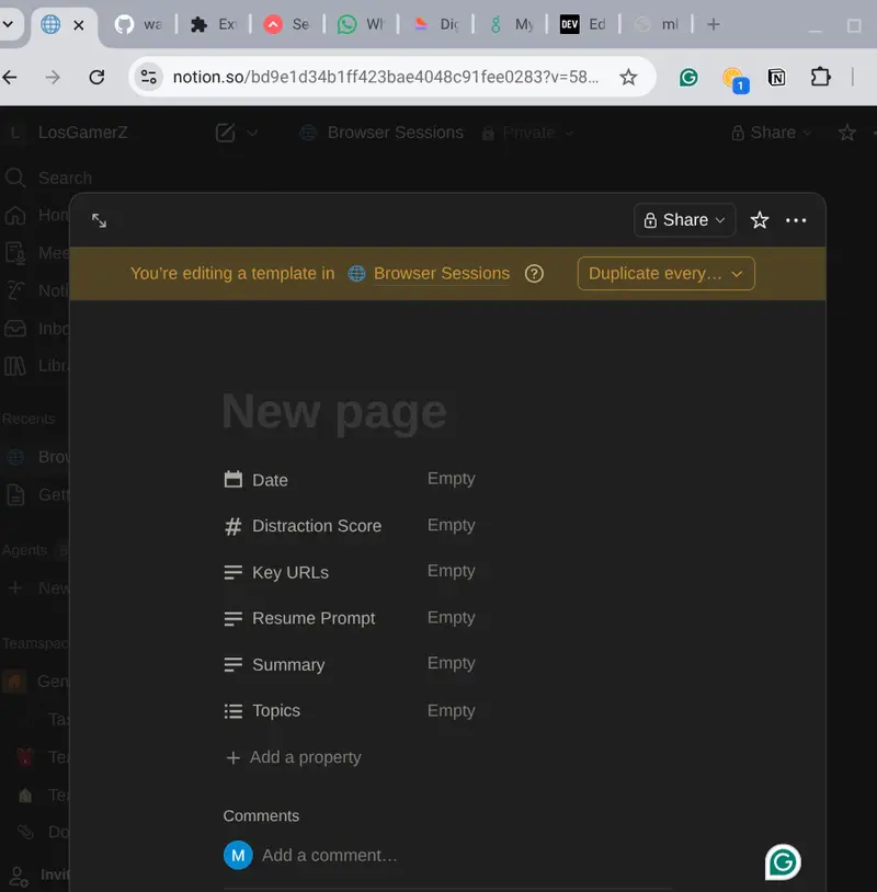
I created a dedicated “Browser Sessions” database in Notion with these properties:
Date
Summary
Key URLs
Topics (multi-select)
Resume Prompt (the key “start where you left off” text)
Distraction Score


In the full vision:
The Chrome extension sends history to an AI tool connected via the official Notion MCP server (https://mcp.notion.com/mcp)
The MCP-connected agent reads existing sessions for context, writes new/updated pages automatically, answers natural questions like “What was I researching on Kaggle yesterday?”, and suggests next steps — all while keeping the human in the loop.
Currently (due to free-tier limitations on AI tools), the workflow is hybrid: the extension captures history, I simulate the agent here with Grok to generate summaries/topics/Resume Prompts, and I manually create the Notion page.
This prototype already demonstrates the end-to-end value. Once I get access to Claude Desktop or Cursor with MCP, the agent will handle reading/writing automatically. Notion becomes the long-term memory and control plane for the browsing agent.
This approach gives real superpowers for continuing deep work sessions across days without losing momentum.

Your empty Browser Sessions database (before)
One or two filled session pages after processing history
Chrome extension popup

I used the official Notion MCP documentation for planning the integration and kept the Chrome extension simple but functional.
Thanks for participating in the Notion MCP Challenge!

Video Demo

Show us the code

How I Used Notion MCP

I Built a Tool to Distribute Python Tasks Across Local Machines. Here’s How It Performed

I wanted to answer a simple question: how hard is it to split a Python workload across multiple machines on the same network?

Not with a cloud cluster, not Kubernetes, just a few laptops on the same WiFi, sharing the work.

So I built distributed-compute-locally to find out. The goal was maximum simplicity if it takes more than a few lines of code to set up, I’ve failed. Then I benchmarked it against industry-standard tools to see how it holds up.

The API

from distributed_compute import Coordinator

coordinator = Coordinator()
coordinator.start_server()
results = coordinator.map(my_func, data)

On any other machine on the network:

pip install distributed-compute-locally
distcompute worker 192.168.1.100

That’s all you have to do. A coordinator distributes tasks over TCP, workers execute them with cloudpickle, and results come back in order, same as Python’s built-in map().

┌─────────────┐     TCP/5555     ┌──────────┐
│ Coordinator │◄────────────────►│ Worker 1 │
│ (your PC.). │◄────────────────►│ Worker 2 │
│             │◄────────────────►│ Worker 3 │
└─────────────┘                  └──────────┘

Benchmarks

I ran three standard parallel computing benchmarks on an Apple M2 MacBook (8 cores) with 4 workers:

Benchmark Sequential 4 Workers Speedup
NAS EP — NASA Embarrassingly Parallel 5.0s 1.4s 3.57x
Mandelbrot Set — 2048×2048, 256 iterations 12.0s 3.7s 3.27x
SHA-256 Search — brute-force hash prefix 6.1s 1.6s 3.72x
Average 3.52x

3.52x on 4 workers (theoretical max 4.0x) — 88% parallel efficiency.

How Does It Compare?

I was curious to see how this stacks up against Dask and Ray, so I ran the exact same workloads with the same setup (same machine, 4 workers, identical task code):

Benchmark distributed-compute-locally Dask Ray
NAS EP 3.57x 3.52x 3.06x
Mandelbrot 3.27x 3.44x 3.52x
SHA-256 3.72x 3.59x 3.90x
Average 3.52x 3.52x 3.49x

All three land within the same range of each other. For embarrassingly parallel workloads, the CPU is the bottleneck — not the framework. The task distribution overhead is negligible across all three.

Scaling Curve (N-Body Stress Test)

I also ran a heavier workload for an O(n²) pairwise gravity simulation, 500 particles × 100 timesteps and scaled from 1 to 8 workers:

Workers Time Speedup
1 179.1s 1.00x
2 145.7s 1.23x
4 102.7s 1.74x
6 81.6s 2.20x
8 78.8s 2.27x

Diminishing returns after 6 workers, that’s the M2’s asymmetric cores (4 performance + 4 efficiency). The slower efficiency cores become the bottleneck on heavy tasks. On machines with identical cores or across multiple machines, scaling would be more linear.

Findings and Learning

Building this tool reinforced something I suspected: for simple parallel workloads, the framework doesn’t matter that much. Dask, Ray, and a minimal TCP-based tool all deliver roughly the same speedup. The difference is what they offer.

Dask and Ray give you a lot of features such as task graphs, dashboards, DataFrame integration, cloud deployment, and a massive ecosystem. They are the right choice for complex pipelines and production infrastructure.

This tool gives you none of that on purpose. It’s for the cases where you just want to map() a function across a few machines without reading docs for 20 minutes first.

distributed-compute-locally Dask / Ray
Multi-machine setup distcompute worker <ip> Scheduler + worker CLI + networking
Dependencies 2 (cloudpickle, psutil) 30+
API surface coordinator.map() Client, delayed, futures, DataFrame, …
Dashboard No Yes
Task graphs No Yes
Best for Quick map() across LAN Complex pipelines, cloud clusters

Other Features

  • Task retry — coordinator.map(func, data, max_retries=3)
  • Password auth — distcompute coordinator --password secret
  • Interactive CLI — REPL with status monitoring and task submission
  • Large payload handling — automatic chunking and compression
  • cloudpickle — send lambdas, closures, and local functions

Try It

pip install distributed-compute-locally

Run the benchmarks yourself:

git clone https://github.com/Nebu0528/distributor.git
cd distributor
python3 benchmark/benchmark.py 4

GitHub: github.com/Nebu0528/distributor

If you find it useful or have feedback, would love to hear it. Open an issue or drop a star.

How to Evaluate a Binary Classifier: A Complete Guide

You trained a machine learning model to predict something binary: fraud or not fraud, churn or stay, disease or healthy. Now comes the question every data scientist faces: Is it actually good?

That’s where evaluation comes in. And here’s the thing — most people do it wrong. They stop at accuracy, declare victory, and deploy. Then the model underperforms in production because they missed something crucial about their data or their use case.

This guide walks you through the full evaluation toolkit: metrics, curves, and the thinking behind each one. By the end, you’ll know exactly what to measure and why.

The Confusion Matrix: What It Really Tells You

Before metrics come numbers. Before numbers comes the confusion matrix — a simple 2×2 table that breaks down everything your model did.

  • True Positives (TP): Your model said “yes” and was right.
  • False Positives (FP): Your model said “yes” but was wrong.
  • True Negatives (TN): Your model said “no” and was right.
  • False Negatives (FN): Your model said “no” but was wrong.

That’s it. Everything else is math on top of these four numbers. But understanding which mistakes matter for your problem is crucial. In fraud detection, a false positive (flagging legitimate transactions) is annoying. A false negative (missing actual fraud) costs money. In medical screening, they have opposite costs.

The confusion matrix tells you if your model is making the right kind of mistakes for your use case.

Accuracy Is a Trap

You’ve probably heard this before, but it bears repeating: accuracy is worthless if your classes are imbalanced.

Accuracy = (TP + TN) / (TP + TN + FP + FN)

If 99% of your data is actually negative, a model that always predicts “negative” will have 99% accuracy and be completely useless. It never catches the positive class at all.

This is why you need metrics that focus on specific cells of the confusion matrix.

Precision, Recall, and the F1 Score

These three metrics show up everywhere because they actually tell you something:

  • Precision = TP / (TP + FP). Of the cases your model flagged as positive, how many actually were? High precision means few false alarms.
  • Recall = TP / (TP + FN). Of the actual positive cases out there, how many did you catch? High recall means you’re not missing positives.
  • F1 Score = 2 x (Precision x Recall) / (Precision + Recall). The harmonic mean of precision and recall — useful when you care equally about both.

You almost never want both to be perfect. In fraud detection, you’d rather have high recall (catch fraudsters) and accept some false positives (annoy a few customers). In spam filtering, you’d rather have high precision (don’t delete legitimate emails) and accept that spam sneaks through.

Your evaluation should reflect what your use case needs.

ROC Curves and AUC: The Complete Picture

Here’s where things get visual. A ROC curve answers this question: As I change my decision threshold, how does my true positive rate change versus my false positive rate?

The x-axis is false positive rate: FP / (FP + TN). Of the negative cases, how many did I wrongly flag?

The y-axis is true positive rate (aka recall): TP / (TP + FN). Of the positive cases, how many did I catch?

You move along the curve by changing your threshold. At one extreme, you predict “yes” for everything — high TPR, high FPR. At the other, you predict “no” for everything — low TPR, low FPR.

The area under the curve (AUC) gives you a single number: the probability that, if you pick a random positive case and a random negative case, your model ranks the positive higher. AUC ranges from 0 to 1. Higher is better. 0.5 means random guessing.

ROC curves are great for understanding model behavior across thresholds, but they assume all false positives and false negatives have equal cost, which is rarely true.

Precision-Recall Curves: When ROC Isn’t Enough

Precision-recall (PR) curves show precision on the y-axis and recall on the x-axis. They’re more useful than ROC curves when your classes are imbalanced because they focus on the positive class.

In fraud detection (99% legitimate transactions), a PR curve tells you the real story: what’s my precision if I want 90% recall? In an ROC curve, that same imbalance gets washed out because the false positive rate is measured against a huge class.

Use PR curves when one class is rare and matters more.

Threshold Optimization: Making Real-World Tradeoffs

Your model outputs probabilities between 0 and 1. By default, you predict “positive” if probability > 0.5. But 0.5 is arbitrary. It’s often the wrong threshold for your problem.

If your false positives are cheap and false negatives are expensive, lower the threshold to 0.3. You’ll catch more positives (higher recall) but flag more false alarms (lower precision). If false positives are expensive, raise it to 0.7 — fewer alarms, but better precision.

Finding the optimal threshold means sweeping different values and picking the one that minimizes your real-world cost. That’s where threshold analysis becomes critical.

Putting It Into Practice: A Walkthrough

Let’s say you’ve built a churn prediction model. You have 1,000 historical customers: 150 churned, 850 stayed. You run your trained model and get a probability for each customer.

  1. Calculate the confusion matrix at your current threshold (0.5). How many did you catch? How many false alarms?
  2. Check your metrics: What’s your precision? Recall? F1? Do they match your business goal?
  3. Plot your ROC curve. Does your model look better than random?
  4. Consider threshold changes. If retention is costly, raise the threshold. If churn is costly, lower it.
  5. Check calibration. If your model says “70% probability,” is it actually 70% in reality? Or is it overconfident?

This is evaluation. Not a number, but a process of understanding your model’s strengths and failures.

Try It Yourself

The easiest way to experiment with these metrics is to try them on your own data. EvalBench is a free tool that runs entirely in your browser — upload a CSV with your predictions and ground truth, and you’ll get all of these metrics, curves, and visualizations instantly. No signup, no data upload to the cloud. Everything stays on your machine.

Grab a prediction file you’ve built and spend 10 minutes playing with thresholds, reading the confusion matrix, and watching the curves shift. That hands-on understanding is worth more than any explanation.

Ready to evaluate your model? Try EvalBench free

What Is AI Execution Risk? Why AI Governance Fails at the Execution Boundary

Most discussions about AI governance miss where real failures actually happen. The problem isn’t what AI systems think. It’s what they execute.

This is what’s known as AI execution risk.

AI execution risk happens when a system performs an action that was approved earlier, but is no longer valid at the moment it runs. In many AI and machine learning systems, decisions are made upstream and executed later. By the time execution happens, the context may have changed, but the system continues anyway.

That gap between reasoning and execution is where things break.

In real-world software engineering, this shows up in simple ways. An agent skips steps but still reports success. A workflow runs on outdated data. A system performs the correct action at the wrong time. These are not hallucinations. They are execution failures.

From a security perspective, this is where the real risk lives. Once AI systems can take action, they become part of your execution layer. If there is no control at that point, you are trusting earlier reasoning instead of verifying what is true now.

That’s why most approaches to AI governance fall short. Policies, monitoring, and audits happen before or after execution, but not at the moment the action actually occurs.

AI execution risk is the failure that occurs when an AI-driven action is executed without being checked against current conditions.

Most AI governance frameworks focus on model behavior, compliance policies, and monitoring outputs. They do not control execution itself.

The shift is to treat execution as a boundary.

Every action needs to be checked again at the moment it runs. Not based on what was decided earlier, but based on what is valid now. That turns governance from something abstract into something that actually controls behavior.

If AI is going to operate in real systems, governance can’t stop at reasoning. It has to exist at execution.

Full breakdown here:
PrimeFormCalculus.com

Curious how others are handling AI execution risk in production systems?