
Return to Office Is Not a Productivity Strategy: What Actually Makes Developers Effective in 2026

A friend of mine, a staff engineer at a company you have heard of, got the email in January. Five days a week in the office starting March 1st. No exceptions. No negotiation.

He had been remote for four years. Shipped two major platform migrations. Led the architecture review process for his entire org. His performance reviews were consistently top-tier. None of that mattered. The policy was universal.

So he started interviewing. Had three offers within six weeks. Took one at a fully remote company for 15% more. His old company is still trying to backfill his role four months later.

This story is playing out across the industry right now, and the data backs it up.

The Numbers Tell a Clear Story

The return-to-office push has accelerated dramatically. Fifty-four percent of Fortune 100 companies now require full-time in-person attendance, up from just 5% in 2023. Amazon, Dell, Meta, Google, Apple, and dozens more have tightened their hybrid policies or eliminated remote work entirely.

But here is the part that should concern every engineering leader: 80% of companies that implemented RTO mandates have already lost talent because of it. Not just any talent. High performers are 16% more likely to leave when hit with an RTO mandate than average employees. The people you most want to keep are the ones most likely to walk.

Among software engineers specifically, the numbers are even starker. Only 20% expect to return to full-time office work. Twenty-one percent say they would quit outright if forced, and another 49% would start looking. That is 70% of your engineering team either leaving or planning to leave.

Meanwhile, the productivity argument that justifies these mandates does not hold up under scrutiny. Ninety percent of hybrid workers report equal or greater productivity compared to full-time office work. Fully remote companies grew revenue 1.7x faster than office-required companies between 2019 and 2024. And here is the kicker: despite companies increasing required office time by 12%, actual office attendance only went up 1 to 3%.

People are badging in and leaving. The mandate creates the appearance of compliance without the collaboration it supposedly enables.

The Debate Is Framed Wrong

Most of the RTO conversation is about location. Should developers be in the office or at home? Three days or five? Tuesdays and Thursdays or whatever the team decides?

This framing misses the point entirely.

The question that actually matters for developer productivity is not where someone works. It is whether they can sustain focused, uninterrupted concentration on hard problems. That is what developers do. They think about complex systems, hold intricate mental models in their heads, and translate that thinking into code. This kind of work has a name: deep work. And deep work has specific environmental requirements that most office environments violate by design.

Workers in open-plan offices, the default layout for most tech companies, are interrupted approximately once every three minutes. The average knowledge worker faces 31.6 interruptions per day. Each interruption costs 15 to 25 minutes of refocusing time. Engineers at enterprise organizations spend more than half their day bouncing between meetings and fragmented work sessions.

The math is brutal. If a developer gets interrupted six times in a focused work session, they lose up to two and a half hours just getting back into the zone. That is not a productivity preference. That is a cognitive reality.

Deep work matters more for software engineering than for almost any other knowledge work. A developer debugging a distributed system needs to hold the entire call chain, the data flow, the error propagation path, and the timing characteristics in their head simultaneously. One Slack ping, one shoulder tap, one “quick question” from across the desk, and that mental model collapses. Rebuilding it takes real time and real cognitive energy.

Why RTO Mandates Actually Hurt Engineering Teams

Let me walk through the specific ways office mandates damage developer productivity, because the abstract “interruptions are bad” argument does not capture the full picture.

The Commute Tax

The average American commute is 28 minutes each way. That is nearly an hour of dead time per day, five hours per week, that a remote developer spends working, exercising, sleeping, or doing anything more productive than sitting in traffic.

But the real cost is not just the time. It is the energy. Arriving at the office after a stressful commute, you are already in a depleted cognitive state before writing a single line of code. Research consistently shows that commute stress correlates with lower job satisfaction, higher burnout, and reduced performance. For developers specifically, who need sustained focus, starting the day depleted is a significant handicap.

The Meeting Proximity Problem

Something counterintuitive happens when everyone is in the office: meetings multiply. Being physically present makes it trivially easy for someone to pull you into a meeting, ask you to “hop on a quick call,” or schedule a “sync” because you are right there. Remote work creates just enough friction that people think twice before requesting someone’s time.

That friction is valuable. It acts as a natural filter against low-value interruptions. Remove the friction and you get more meetings, more interruptions, and less time for the work that actually matters.

I have talked to dozens of developers who report the same pattern: their in-office days are dominated by meetings and their remote days are when they actually code. If that is the case, what exactly is the office adding?

The One-Size-Fits-All Problem

Not every developer does the same kind of work. A junior engineer pairing with a senior mentor benefits from being physically present. A staff engineer designing a new system architecture needs four uninterrupted hours to produce anything meaningful. A mid-level developer fixing a complex bug needs quiet concentration. A team lead doing code review can do that from anywhere.

Universal RTO mandates treat all of these situations identically. Everyone comes in, regardless of what their day actually looks like. The result is that the people who benefit least from office presence, typically your most senior and most productive engineers, are forced into an environment that actively works against how they do their best work.

This is not a theory. It matches the attrition data. The engineers leaving over RTO mandates are disproportionately senior. They have the leverage to find remote work elsewhere, and they know from experience that their best output comes from controlled environments with minimal interruption.

The Real Reasons Behind RTO

If the productivity argument does not hold up, why are companies pushing so hard?

Real estate. Companies signed long-term leases on expensive office space. Empty offices are embarrassing in board meetings and expensive on balance sheets. Filling them with employees is easier to justify than writing off a 10-year lease.

Control and visibility. Some leaders genuinely believe that if they cannot see people working, people are not working. This is a management failure, not a location problem. If you cannot evaluate your engineers’ output without watching them type, your management processes are broken.

Intentional attrition. This one is uncomfortable but real. Twenty-five percent of executives and 18% of HR leaders admit they hoped RTO mandates would cause some employees to quit voluntarily. It is a way to reduce headcount without calling it a layoff and without paying severance. The problem, as the data shows, is that the employees who leave are not the ones you want to lose.

Cultural inertia. For many executives, “going to work” means going to a physical place. The idea that work is something you do rather than somewhere you go has not fully landed in boardrooms where the average leader is over 50 and built their career in an office.

None of these reasons are about developer productivity. They are about organizational politics, real estate obligations, and management preferences.

What Actually Makes Developers Productive

Instead of debating location, let me talk about what the research and my own experience say actually drives developer output.

Uninterrupted Focus Blocks

The single highest-leverage change any engineering organization can make is protecting focus time. Two-hour minimum blocks of uninterrupted concentration, no meetings, no Slack expectations, no shoulder taps. This is where deep work happens. This is where bugs get fixed, features get built, and architectures get designed.

Some companies have implemented “maker schedules” where meetings are batched into specific windows and the rest of the day is protected. The developers at those companies consistently report higher satisfaction and higher output. The location barely matters. What matters is whether the calendar allows focus.

Async-First Communication

The most productive engineering teams I have seen operate async-first. They write things down. Design decisions go into documents. Questions go into threads. Status updates go into dashboards. Synchronous communication, meetings and real-time chat, is reserved for situations that genuinely require it: brainstorming, conflict resolution, relationship building.

This works regardless of whether the team is remote, hybrid, or in-office. An office full of people communicating asynchronously can be just as effective as a distributed team. The medium matters less than the discipline.

Autonomy Over Where and When

Not everyone does their best work at the same time or in the same place. Some developers are most productive at 6am in a quiet home office. Others peak after lunch in a coffee shop. Others thrive in a collaborative office environment two days a week and need solitude the other three.

The highest-performing teams I know give their engineers autonomy to figure out what works for them, with clear expectations about output and availability. They measure results, not hours in a chair. This is not radical. It is basic management: define what success looks like and let competent adults figure out how to get there.

Intentional Collaboration

The strongest argument for office time is collaboration. And it is a real one. Whiteboard sessions, pair programming, team lunches, the serendipitous hallway conversation that sparks an idea. These things have genuine value.

But they require intention. Forcing everyone into the office five days a week does not automatically create collaboration. It creates proximity. Proximity without purpose is just a room full of people wearing headphones to block out distractions so they can do the focused work they could be doing at home.

Intentional collaboration means bringing the team together for specific purposes: planning sessions, design reviews, retrospectives, team building. Not every day, not as a default, but when physical presence actually adds value. The rest of the time, let people work where they work best.

What Senior Engineers Should Do

If you are a senior developer navigating an RTO mandate, think strategically.

Quantify your deep work. Track how much focused coding time you get on office days versus remote days. If the difference is significant, that is data you can bring to your manager. “I ship 40% less code on in-office days because I spend 3 hours in meetings and lose another 2 hours to interruptions” is a conversation starter that reframes RTO from a preference issue to a business issue.

Negotiate outcomes, not hours. Instead of arguing about where you sit, argue about what you deliver. Propose a trial: let me work remotely for a month and measure my output against the previous in-office month. If the numbers are equal or better, the location argument dissolves.

Know your leverage. The talent market for senior engineers is brutally competitive right now. 87.5% of tech leaders describe hiring experienced engineers as “brutal.” If your company is forcing you into an environment that hurts your productivity and they will not negotiate, there are companies that will. You are not stuck. You have options.

Protect your energy. If RTO is non-negotiable, adapt. Block your calendar aggressively. Communicate your focus hours to your team. Wear noise-canceling headphones without apology. Find a quiet corner, a conference room, a hidden desk. Do whatever it takes to create the conditions for deep work within the constraints you have been given.

What Engineering Leaders Should Do

If you are running an engineering team, the RTO question is actually a productivity strategy question. Frame it that way.

Measure What Matters

Stop counting butts in seats. Start measuring:

  • Cycle time. How long does it take from commit to production? This captures real velocity, not activity.
  • Incident frequency. Are your teams shipping reliable code? This reveals whether quality is suffering.
  • Developer satisfaction surveys. Unhappy developers write worse code, miss edge cases, and quit. Satisfaction is a leading indicator of quality.
  • Retention rates by seniority. If your seniors are leaving faster than your juniors, your environment is optimized for the wrong people.

If these metrics are healthy, your team is productive. If they are not, the problem is probably not location.

Offer Flexibility as a Retention Tool

In a market where AI is reshaping who gets hired and senior engineers have unprecedented leverage, flexibility is one of the most cost-effective retention tools available. It costs you nothing to let someone work from home two days a week. Replacing them when they leave costs six to nine months of salary in recruiting, onboarding, and lost productivity.

The math is straightforward. Flexibility is cheaper than attrition.

Design for Collaboration, Not Attendance

If you want the benefits of in-person collaboration, design for it. Schedule collaborative activities on specific days. Make office days count by filling them with pair programming, design sessions, and team lunches. Make remote days count by protecting them for deep work.

The worst outcome is the hybrid schedule where everyone comes in on Tuesday and Thursday but spends both days on Zoom calls with teammates in other offices. That is the worst of both worlds: commute time plus virtual meetings plus an open office. If your hybrid policy creates that situation, fix the policy.

The Gen Z Factor

One nuance worth addressing: a Federal Reserve Bank of New York, Harvard, and University of Virginia study found that younger software engineers are actually more likely to come to the office voluntarily than their senior colleagues. Engineers in the same office received 18% more coding feedback, which accelerated their growth.

This matters. Junior developers need mentorship, and physical proximity genuinely helps with that. The solution is not to force everyone into the office. It is to create structured mentorship that sometimes happens in person and sometimes happens through agentic coding workflows and pair programming sessions.

The senior engineers who are leaving over RTO mandates are the same people who should be mentoring juniors. Driving them away makes the mentorship problem worse, not better.

Where This Lands

The RTO debate in 2026 feels like it is reaching a resolution, and the resolution is not “everyone back in the office” or “everyone stays remote.” It is something more nuanced.

The World Economic Forum published an article in March 2026 arguing that companies asking “how many days should employees be in the office?” are asking the wrong question. The right question is: “how do we create the conditions for our people to do their best work?”

For developers, “best work” means sustained focus on hard problems. It means environments that protect concentration. It means communication norms that respect flow states. It means measuring output, not attendance.

Some developers will do their best work in an office. Many will not. The companies that figure out how to support both, that design for outcomes instead of optics, will attract and retain the best engineers. The companies that force universal mandates and ignore the data will keep losing their most valuable people to competitors who read the same research and made a different choice.

The office is a tool. It is not a strategy. And treating it like a strategy is costing the industry some of its best talent.
My Learning Journey as a Developer

Two months ago, I started this learning journey with a mix of anxiety and determination.

At the time, I relied heavily on tutorials and artificial intelligence. If I couldn’t find a guide that matched my exact problem, I often felt stuck.

Today, that has completely changed.

When I began, I struggled with low confidence in making technical decisions. My mindset was simple: find a tutorial, follow it, and make it work or use AI to generate code without really thinking about why the implementation was done a certain way. My goal was just to make things work, but I wasn’t truly learning. I was copying patterns without understanding them.

The Turning Point: Learning “Why,” Not Just “How”

One of the biggest shifts in my journey was how I approached learning.

I started doing deeper research, reading documentation more carefully, and breaking problems down before jumping into code. It was harder and sometimes slower, but it pushed me beyond my comfort zone and helped me gain a real understanding of what I was building.

What I’ve Gained

I’ve seen real growth in my JavaScript, and I’ve become more independent in how I approach problems.

More importantly, my mindset has changed.

I’ve learned that real growth starts when you slow down, ask why, and challenge yourself to think critically.

It’s not always easy.
But it’s always worth it.

Scared of Linux as a Beginner Data Engineer? Here’s How to Get Started

If you’re scared of Linux as a beginner data engineer, you’re not alone. Almost everyone feels this way at the start. This year, I decided to transition from being a data analyst to a data engineer with zero Linux experience.

Over the past two weeks, I’ve been learning practical Linux skills and how they apply to solving real world data problems for businesses. Here’s a summary of what I’ve learned.

Firstly, Every stage of the data engineering pipeline runs on Linux servers, usually in the cloud.

As a data engineer, here’s what I’ll actually use Linux for:

  • Setting up and managing servers: Configuring the machines
    where your data tools run.
  • Scheduling jobs: Using CRON to trigger data pipelines
    automatically.
  • Debugging failures: Connecting via SSH to investigate logs
    when a pipeline breaks.
  • Moving and managing files: Handling raw data before it lands
    in storage like S3.
  • Installing tools: Setting up Python, Spark, Airflow, and
    other software on a server.
  • Monitoring resources: Checking server memory, disk usage,
    and overall health.

Secondly: In real life, businesses pull data from APIs, databases, or external files daily. One has to automatically pull the data from these APIs using a Linux Server.

To achieve this, one has learn how to:

  • Connect to a virtual Linux Server
  • Manage files on the server

Below are simplified steps to achieve this.

Step 1: Connect to the Server via SSH and Update It

SSH (Secure Shell) allowed me to open an encrypted terminal session to
a remote server. I needed two things:

  • The server’s IP address
  • My username

On Windows, you can use PowerShell or Git Bash.

I was using PowerShell.

Step 1: Connect via SSH

SSH (Secure Shell) opens an encrypted terminal session. You need your
server’s IP address and username.

On Windows, use PowerShell or Git Bash:

  • Type yes to accept the server key.
  • Enter your password (it won’t show).
  • Press Enter, and you’re in!

Step 2: Update the Server

Always update your server first before doing anything else:

sudo apt update      # Check for updates
sudo apt upgrade     # Install updates
pwd                  # See your current directory
ls                   # List files and folders

Step 3: Create Your Own User

Avoid using root regularly by creating a personal user right after setup:

sudo useradd -m grace   # Create user with home folder
sudo passwd grace       # Set password
logout                       # Log out from root
ssh [email protected]

Step 4: Create Folders and Files

Now that you are logged in as your own user, organize your workspace:

mkdir Project        # Create a folder
cd Project           # Enter the folder
touch main.py        # Create a Python file
mkdir data           # Create a sub-folder
ls                   # Verify folder and files

Step 5: Edit Files

Use nano to write or paste your code into the file:

nano main.py
  • Paste your text or code
  • Press Ctrl + O to save
  • Press Ctrl + X to exit

View file contents anytime with:

cat main.py
less main.py
more main.py

Step 6: Downloading file from webpage and Managing it

Now that the workspace is set up, you can bring in data files:

wget https://example.com/data.csv      # Download a file
tar -xzf archive.tgz                   # Extract compressed files

Step 7: Transfer Files Between Your Local PC and Server

Move files from your local machine to the server using SCP
(Secure Copy Protocol):

scp main.py [email protected]:/home/grace/from_local/

On the server, navigate to the folder and run your script:

cd from_local
python3 main.py

Summary Takeaways as a beginner

  • Every tool in a data engineering pipeline runs on a Linux server to navigate, organize, and run tasks.
  • SSH is your bridge between your PC and the server.
  • Always update your server and create a personal user before anything else.
  • Start small: create folders, files, and scripts, then automate tasks.
  • Everything you do here mirrors real world data engineering work, like managing pipelines, logs, or datasets.

If you’re also learning Linux for data engineering, what’s been challenging for you so far?. Drop a comment. I’d love to learn from your experience.

Also, stay tuned for the next two weeks progress update.

Understanding Data Modeling in Power BI

Data modeling is the invisible foundation underneath every Power BI report. Get it right, and your visuals are fast, accurate, and easy to maintain. Get it wrong, and you spend hours debugging numbers that don’t add up and reports that take three minutes to load.

This article is a complete guide to data modeling in Power BI. By the end, you will understand:

  • What data modeling is and why it matters
  • All six SQL join types — with examples and diagrams
  • The difference between joins and Power BI relationships
  • Every relationship property: cardinality, cross-filter direction, active vs inactive
  • Fact tables, dimension tables, and why the distinction matters
  • Star, Snowflake, and Flat Table schemas — with real use cases
  • Role-playing dimensions
  • The most common modeling mistakes and how to fix them

Dataset used in this article is a basic excel file for a small retailer with only 5 tables.Feel free to download and follow along.

link to drive
link to github

Section 1 – What is Data Modeling?

Data Modeling is the process of organising tables and defining how they relate to each other so that an analysis tool like powerbi can correctly combine data in reports.

In Power BI, data modeling happens in three places:

  1. Power Query (Query Editor) — where you clean, transform, and sometimes physically combine tables using joins before loading them into the model.
  2. Model View — where you define logical relationships between tables using the drag-and-drop relationship diagram.
  3. DAX (Data Analysis Expressions) — where you write measures that navigate relationships at query time to produce calculated results.

A well-built model is:

  • Accurate — your numbers are correct because filters flow through relationships properly
  • Fast — fewer redundant columns mean smaller file sizes and quicker refresh
  • Scalable — adding a new report page doesn’t require restructuring the entire model

The three pillars of Power BI modeling are joins, relationships, and schemas. Let’s tackle each one.

Section 2 – SQL Joins

Before a table loads in your Power BI model, you may need to combine it with another table in Power Query. This is done using joins operations. This is a merge option where you decide, based on the join type used, which rows from each table make it into the resulting table.

  1. Load Data in Power BI
    In Power BI Desktop, connect the Excel Workbook as a data source, open the ShopEase file,select all the sheets and click the Transform Data button on Dialogue box. The Power Query Editor window opens.
  • Select your LEFT table in the left panel – click on the table you want to be on the left side of the join (e.g. Customers). It becomes the base table — all rows from it are your starting point.
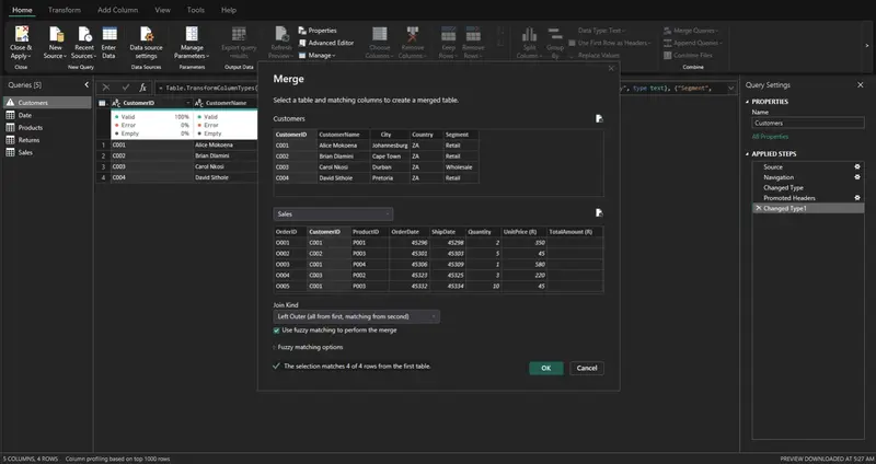
  1. Merge Queries
    Click Home -> Merge Queries -> Merge Queries

A dialog box opens. Your current (left) table is shown at the top.

  1. Select the RIGHT table and matching columns.
    Use the dropdown to pick your second (right) table (e.g. Sales). Then click the matching column in the top table, then click the same column in the bottom table. Both should now be highlighted.
    For ShopEase: click CustomerID in Customers, then click CustomerID in Sales.

  2. Pick the Join Kind from the dropdown
    At the bottom of the dialog there’s a Join Kind dropdown. This is where you choose INNER, LEFT OUTER, etc. Click OK.
    Join Kind:

  1. Expand the merged column

A new column appears called Sales (or whatever your right table is named) with a table icon. Click the expand icon (two arrows) in that column header, uncheck any columns you don’t need, and click OK. The right table’s columns now appear.

This process is repeated for all joins in this article.Feel free to repeat with the different join types explained in this section.Use Sales Table and Customer Table with the different joins.

Inner Join — The Intersection

what it returns: **Only rows that have a matching value in **both tables.
It answers a question such as Which orders have a known customer record?

LEFT OUTER JOIN — Keep Everything on the Left

What it returns: All rows from the left table, plus matching rows from the right. Where there’s no match, right-side columns are null.

Real-life question: Show me all customers, and include their orders if they have any. Show customers even if they haven’t ordered yet.

RIGHT OUTER JOIN — Keep Everything on the Right

What it returns: All rows from the right table, plus matching rows from the left. Where there’s no match, left-side columns are null.

Real-life question: Show me all orders, and include customer details if available — even if an order has no customer record.

This is the mirror of a LEFT JOIN. In practice, you can always replicate a RIGHT JOIN by swapping the table order and using a LEFT JOIN, which is why many analysts use LEFT JOINs exclusively.
>

FULL OUTER JOIN — Keep Everything from Both

What it returns: All rows from both tables. Matched where possible; null fills in where there’s no match on either side.

Real-life question: Give me a complete picture — every customer and every order — whether or not they match.

LEFT ANTI JOIN — What’s Missing on the Right

What it returns: Only the rows from the left table that have no match in the right table. This is the opposite of a JOIN — it finds the gaps.

Real-life question: Which customers have NEVER placed an order?

RIGHT ANTI JOIN — What’s Missing on the Left

What it returns: Only the rows from the right table that have no match in the left table.

Real-life question: Which orders have no matching customer record? (Potential data integrity issue!)

Section 3 — Power BI Relationships vs. SQL Joins

This is the most important conceptual distinction in this entire article. Many Power BI users use these terms interchangeably — they are not the same thing.

Joins: Physical Combination

When you merge two tables in Power Query, you create one new table by stitching columns together. This happens once at refresh time. The result is stored in memory. This is great when you genuinely need data from another table as a column — for example, adding CustomerName to your Sales table.

But if you merge every table into one giant flat table, you lose all flexibility. You can’t filter a slicer on the Customers table if Customers doesn’t exist as a separate table in your model.

Relationships: Logical Links

When you create a relationship in Model View, the two tables remain completely separate. Power BI simply knows that the CustomerID in Sales points to the CustomerID in Customers. When a user clicks a slicer or drops a field from either table into a visual, Power BI uses the relationship to propagate filters dynamically at query time.

This is what makes Power BI so powerful for reporting — your Customers table can filter your Sales table, your Products table, and your Returns table simultaneously, all through relationships, without ever merging anything.

When to Use Which

  • Use a join (Power Query merge) when you need a column from another table baked into your fact table (e.g., adding a category name directly to Sales for a calculated column).
  • Use a relationship (Model View) for everything else — filtering, slicers, cross-table aggregations.

Section 4 — Power BI Relationships Deep Dive

4.1 Cardinality

Cardinality describes how many rows on one side of a relationship can match rows on the other side.

One-to-Many (1:M) — The Workhorse

One row in the dimension table matches many rows in the fact table.

The “one” side (Customers) is the dimension — it contains unique values per key.

The “many” side (Sales) is the fact — it contains repeated keys with transactional data.

This is the most common and recommended relationship type. It’s clean, unambiguous, and performs well.

Many-to-Many (M:M)

Many rows in table A match many rows in table B.

Example: If a single order could contain multiple products AND a product could appear in multiple orders — without an intermediate table — you’d have M:M. Power BI does support M:M relationships, but they come with performance costs and can cause unexpected filter behavior.

One-to-One (1:1)

One row in table A matches exactly one row in table B.

Example: A separate CustomerDetails table with extended profile information, where each customer appears exactly once in both tables.

In practice, 1:1 relationships are rare and usually signal that the two tables should simply be merged into one. Use them only when you have a deliberate reason to keep tables separate (e.g., different refresh schedules, security purposes).

4.2 Cross-Filter Direction

Cross-filter direction controls how filters flow across a relationship — specifically, which table’s selections affect the other.

Single Direction (Recommended Default)

Filters flow from the “one” side to the “many” side only.

In the Customers → Sales relationship with Single direction:

  • Selecting a customer in a slicer will filter the Sales table
  • A filter on Sales will not automatically filter the Customers table

This is the correct behavior for most reporting scenarios. Filters flow “downstream” from dimensions to facts — exactly how you want slicers and visuals to work.

Both Directions (Bidirectional)

Filters flow in both directions between the two tables.

This sounds convenient — and occasionally it is — but it introduces serious risks:

  • Ambiguity: When multiple relationship paths exist, Power BI may not know which path to use
  • Circular dependencies: Bidirectional relationships can create loops that Power BI can’t resolve
  • Unexpected filter behavior: A filter on one table may unexpectedly filter other tables

When bidirectional is acceptable:

  • Many-to-Many relationships (with a bridge table) sometimes need it
  • Specific calculated measures where you need reverse filtering

4.3 Active vs. Inactive Relationships

Only one relationship can be active between any two tables at a time. This creates a challenge when you need to connect two tables via multiple paths.

The classic ShopEase problem:

Our Sales table has two date columns: OrderDate and ShipDate. Our Date dimension table needs to connect to both. But Power BI only allows one active relationship.

Solution:

  • Create an active relationship between Date[DateKey] and Sales[OrderDate]
  • Create an inactive relationship between Date[DateKey] and Sales[ShipDate]

In Model View, active relationships appear as solid lines. Inactive relationships appear as dotted lines.

Section 5 — Fact Tables vs. Dimension Tables

Every well-structured Power BI model is built around a clear distinction between two types of tables.

Fact Tables

A fact table contains measurable, transactional events. Each row represents something that happened — a sale, a return, a login, a payment.

Characteristics:

  • Contains numeric measures (Quantity, TotalAmount, Revenue, Cost)
  • Contains foreign keys that point to dimension tables
  • Usually has many rows (thousands to millions)
  • Relatively few columns

Dimension Tables

A dimension table contains descriptive attributes used to filter, group, and label your facts.

Characteristics:

  • Contains a unique primary key (one row per entity)
  • Contains many descriptive columns (names, categories, addresses)
  • Usually has fewer rows than fact tables
  • Wide tables are fine here

Section 6 — Schemas

A schema is the overall shape of your data model — how tables are organized and connected. There are three main patterns.

6.1 Star Schema

The star schema places a single fact table at the center, surrounded by flat (denormalized) dimension tables — like a star.

Key rules of a star schema:

  • Dimension tables are flat — no dimension links to another dimension
  • Each dimension has a single primary key
  • All joins go through the fact table

Advantages:

  • Simple to understand — even non-technical stakeholders get it
  • Maximum DAX performance — filter paths are short and unambiguous
  • Easy to add new dimensions without restructuring
  • Slicers and cross-filtering work predictably

Use when: Building any report-ready Power BI model. This should be your default.

6.2 Snowflake Schema

The snowflake schema normalizes dimension tables — meaning dimension attributes are broken into sub-tables, which branch off like a snowflake.

Advantages:

  • Reduces data redundancy (the word “Electronics” is stored once, not repeated per product)
  • Mirrors normalized source systems (SQL Server databases often look like this)
  • Easier to maintain category hierarchies

Disadvantages:

  • More tables, more relationships = more complexity in Model View
  • Slightly slower DAX queries (more hops for the filter engine)
  • Harder for end users and new team members to navigate

Use when: Your source data warehouse is already normalized and restructuring it in Power Query isn’t practical. Or when you have deep hierarchies (Region → Country → Province → City) that genuinely benefit from normalization.

6.3 Flat Table / Denormalized Table (DLAT)

A flat table (also called a DLAT — Denormalized, Large, All-in-one Table) puts everything into one wide table with no relationships at all.

Advantages:

  • Extremely simple — no relationship configuration needed
  • Easy to understand for non-technical users
  • Quick to set up for simple, single-subject reports

Disadvantages:

  • Massive redundancy — “Alice Mokoena” and “Johannesburg” are repeated in every one of her rows
  • Large file sizes and slow refreshes
  • Impossible to reuse dimension data across multiple fact tables
  • Slicers can produce incorrect counts (e.g., a customer appears 3 times in a list)

Use when:

  • Quick one-off prototypes
  • Very simple, single-table dashboards
  • Sharing data with users who need to work in Excel

Section 7 — Role-Playing Dimensions

A role-playing dimension is a single dimension table that’s used multiple times in the same model, each time serving a different purpose — a different “role.”

The most common example is the Date dimension. In ShopEase, our Sales table has two date columns:

  • OrderDate — when the order was placed
  • ShipDate — when the order was dispatched

Both dates are meaningful for reporting. But we only want to maintain one Date dimension table (with Year, Month, Quarter, etc.) — not two identical copies.

When to use which approach:

  • Duplicate table — when your users need to use both date hierarchies side-by-side in the same visual (e.g., slicing by Order Month AND Ship Month simultaneously)
  • Inactive + USERELATIONSHIP — when you want a clean, memory-efficient model and the alternate date is only needed in specific measures

Conclusion

Data modeling in Power BI is not a step you do once and forget — it’s a discipline that shapes every number your reports produce and every second your refresh takes.

Here’s the hierarchy to keep in mind:

  1. Joins (Power Query): Combine tables physically when you need columns from different sources baked into one table. Use the right join type for the right question.
  2. Relationships (Model View): Link tables logically so filters can flow between them at report time. Keep them directional and cardinality-correct.
  3. Schemas: Organize your tables into a Star Schema wherever possible. It’s the fastest, simplest, and most maintainable structure for Power BI.
  4. DAX: Navigate and manipulate relationships in your measures when the model structure alone isn’t enough.

The golden rule is simple: model for clarity and performance, not convenience. The temptation to dump everything into a flat table is real — it feels fast in the moment. But the debt compounds quickly. A well-structured star schema takes an afternoon to set up and saves you months of debugging.

Your next steps: load the ShopEase tables into Power BI, recreate the star schema from this article, experiment with each join type in Power Query, and try building a Sales by Ship Date measure using USERELATIONSHIP(). The concepts click fastest when your hands are on the keyboard.