Sending beautiful Playwright test reports via email using shadcn/ui and react-email
Why email reports?

After a CI run finishes you usually have two options: check GitHub Actions manually or wait for a Slack ping with a link. Neither is great when you want the whole team — including non-engineers — to see what broke.

@playwright-labs/reporter-email solves this by hooking into Playwright’s reporter API and sending an HTML email as soon as the run completes. No extra server, no external service — just SMTP.

New in this release: shadcn/ui templates

The package now ships 4 new templates built on top of email-safe shadcn/ui components.

“Email-safe” means no Radix UI (requires browser APIs), no CSS variables (not supported in most clients), and <a> tags instead of <button> for interactive elements.

Template overview

Template Import Key feature
Base …/shadcn Badge + Card layout
Chart …/shadcn/base-chart Pass-rate stacked bar
Button …/shadcn/base-button CTA links to report / failures
Themes …/shadcn/base-themes 6 color themes
Select …/shadcn/base-select Status filter

Subpath exports

Each template ships as its own bundle so you only import what you use:

import { PlaywrightReportShadcnChartEmail }
  from "@playwright-labs/reporter-email/templates/shadcn/base-chart";

TypeScript resolves types correctly with "moduleResolution": "bundler" in tsconfig.json.

Quick setup

Install the package:

npm install @playwright-labs/reporter-email

Add to playwright.config.ts:

import type { PlaywrightTestConfig } from "@playwright/test";

const config: PlaywrightTestConfig = {
  reporter: [
    ["@playwright-labs/reporter-email", {
      host: "smtp.example.com",
      port: 587,
      from: "[email protected]",
      to: ["[email protected]"],
      template: "shadcn",          // or "shadcn-chart", "shadcn-themes", …
      statusFilter: ["failed"],    // send only failures
    }],
  ],
};

export default config;

The templates

The most useful pattern for busy pipelines: send an email only when something breaks, and show only the failed tests.

import PlaywrightReportShadcnEmail from
  "@playwright-labs/reporter-email/templates/shadcn/base-button";

<PlaywrightReportShadcnEmail
  result={result}
  testCases={testCases}
/>

The email renders a shadcn-like button trigger showing.

Previewing templates locally

The examples/ directory has a dev server powered by react-email:

cd packages/reporter-email/examples
pnpm email:preview
# → http://localhost:3000

In your project:

# install @react-email/components & @react-email/render 
pnpm i @react-email/components @react-email/render -D

Create template & Start dev server

mkdir -p ./emails
pnpm exec email dev --dir emails

Create your template:

import React from "react";
import type { FullResult, TestCase, TestResult } from "@playwright/test/reporter";
import PlaywrightReportEmail from "@playwright-labs/reporter-email/templates/base";

// mock data
const result = {
  status: "failed",
  duration: 14_320,
  startTime: new Date(),
} satisfies FullResult;

function tc(title: string, suite: string): TestCase {
  return { title, parent: { title: suite } } as unknown as TestCase;
}

function tr(status: TestResult["status"], duration: number): TestResult {
  return { status, duration } as TestResult;
}

const testCases: [TestCase, TestResult][] = [
  [tc("Login with valid credentials",   "Auth"),          tr("passed",  342)],
  [tc("Login with invalid credentials", "Auth"),          tr("passed",  289)],
  [tc("Logout",                         "Auth"),          tr("passed",  190)],
  [tc("Add item to cart",               "Shopping Cart"), tr("failed", 5102)],
  [tc("Remove item from cart",          "Shopping Cart"), tr("failed", 4320)],
  [tc("View product details",           "Product"),       tr("passed",  421)],
  [tc("Filter by category",             "Product"),       tr("passed",  374)],
  [tc("Search by keyword",              "Search"),        tr("skipped",   0)],
];

// your template!
/** Default export is required by the React Email dev server. */
export default function PlaywrightReportPreview() {
  return (
     <>
      <span> This is an example preview</span>
    <PlaywrightReportEmail result={result} testCases={testCases} />
     </>
  );
}

Check out the repo for all preview files and the full source.

GitHub: https://github.com/vitalics/playwright-labs

Pulse & Precedent: A Living Timeline of Gender Equity

This is a submission for the 2026 WeCoded Challenge: Frontend Art

Show us your Art

Live Demo

Inspiration

For the #WeCoded 2026 challenge, I wanted to create more than just a timeline. I wanted to build a digital relay race.
My project, Pulse & Precedent, is an interactive archive that honors the pioneers of gender equity while passing the torch to the next generation of developers and advocates.

🕊️ A Note to the Community
To my fellow underrepresented developers: Our stories are data points in a larger constellation. Every PR you submit and every junior dev you mentor adds a “pulse” to this archive.

My Code

Building this was a journey in balancing interactivity with meaningful storytelling.

I used Google AI Studio as my primary architectural partner. It helped me move from a static grid to a dynamic Constellation UI, where voices like Malala Yousafzai and Radia Perlman float like stars in a galaxy of progress.

I utilized React, Tailwind CSS, and Framer Motion to create a lens interaction. When you hover over a name, the animation locks, the element glows, and their story emerges from the blur.

One of my biggest hurdles was making the Echo Chamber feel organic. AI Studio helped me refine the jittered grid logic to ensure the floating elements felt alive without overlapping.

The most rewarding part was coding the Action Cards. I realized that looking at history is only half the battle. We have to act on it. I integrated specific triggers for:

  • Accessibility Audits: Because equity starts with access.
  • Empathetic Code Reviews: To ensure our technical spaces remain supportive.

📂 GitHub Repo

Your Pipeline Is 16.3h Behind: Catching Human Rights Sentiment Leads with Pulsebit

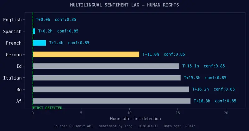
English coverage led by 16.3 hours. Af at T+16.3h. Confidenc

Your Pipeline Is 16.3h Behind: Catching Human Rights Sentiment Leads with Pulsebit

We recently uncovered a compelling anomaly: a 24-hour momentum spike of -1.243 around the topic of human rights. This negative momentum indicates a notable shift in sentiment, leading to a cluster of articles focused on the FIFA World Cup being held amid a “human rights crisis” in the US, as reported by Al Jazeera. With 16.3 hours of lead time in English press coverage, this spike reveals just how quickly sentiment can shift, and how crucial it is for us to stay on top of these developments.

The Problem

Your model missed this by 16.3 hours. This significant lead time underscores a structural gap in any pipeline that doesn’t effectively account for multilingual origins or dominant entities. In this case, English-language articles were driving the narrative, and if your approach relies solely on a single language or fails to recognize the dominant entities, you’re left behind. The implications are clear: failing to capture this sentiment shift could mean missing out on critical insights and opportunities for timely decision-making.

English coverage led by 16.3 hours. Af at T+16.3h. Confidenc
English coverage led by 16.3 hours. Af at T+16.3h. Confidence scores: English 0.85, Spanish 0.85, French 0.85 Source: Pulsebit /sentiment_by_lang.

The Code

Here’s how we can catch this anomaly using our API. First, we’ll filter by language to focus on English articles. Then, we’ll run the cluster reason string through the sentiment scoring endpoint to assess the narrative’s framing.

import requests

# Step 1: Geographic origin filter
response = requests.get(
    'https://api.pulsebit.com/v1/sentiment',
    params={
        'topic': 'human rights',
        'lang': 'en',
        'momentum': -1.243
    }
)

![Geographic detection output for human rights. France leads w](https://pub-c3309ec893c24fb9ae292f229e1688a6.r2.dev/figures/g3_geo_output_1774928363707.png)
*Geographic detection output for human rights. France leads with 1 articles and sentiment -0.75. Source: Pulsebit /news_recent geographic fields.*


data = response.json()
print(data)

# Step 2: Meta-sentiment moment
cluster_reason = "Clustered by shared themes: least, dead, haiti, massacre, human."
meta_sentiment_response = requests.post(
    'https://api.pulsebit.com/v1/sentiment',
    json={'text': cluster_reason}
)

meta_sentiment_data = meta_sentiment_response.json()
print(meta_sentiment_data)

In this code, the first API call filters sentiment data specifically for English articles about human rights, identifying the negative momentum we observed. The second call processes the cluster reason, giving us insight into how the narrative is framed around the concepts of “least,” “dead,” “Haiti,” and “human.” This is where our analysis gets its depth, allowing us to understand not just the surface-level sentiment but the underlying themes driving it.

Left: Python GET /news_semantic call for 'human rights'. Rig
Left: Python GET /news_semantic call for ‘human rights’. Right: returned JSON response structure (clusters: 3). Source: Pulsebit /news_semantic.

Three Builds Tonight

Here are three specific builds we can implement based on this pattern:

  1. Signal Detection: Set up a signal that triggers an alert when the sentiment score for “human rights” drops below -0.5 with a momentum threshold of -1.243. This ensures you’re alerted to significant downward shifts in sentiment.

  2. Geo-Filtered Analysis: Create a dashboard that visualizes sentiment trends for “human rights” across different geographic locations, specifically filtering for English-language content. This way, you can spot regional variations in sentiment early.

  3. Meta-Sentiment Loop: Implement a system that automatically fetches cluster reasons for articles with significant sentiment shifts and runs them through the sentiment endpoint. This will help you continuously refine your understanding of the narrative around specific topics like human rights, especially as new stories emerge and old ones fade.

Get Started

Ready to dive in? Check out our documentation for guidance. With just a few lines of code, you can start capturing insights like these in under 10 minutes.

AI-powered PostgreSQL observability

pg-collector streams live PostgreSQL telemetry into a 7-dimension state machine that predicts failures, detects query regressions, and answers the 5 questions every DBA asks — automatically.

Is my database healthy?
Single-sentence verdict with confidence level, time-in-state, and 7-dimension breakdown. No interpretation needed.

What changed?
Causal narrative linking state transitions to query regressions, workload shifts, and configuration changes with timestamps.

What will break next?
Ranked risk register with ‘days to breach’ projections. Vacuum wraparound in 18 days. Connection exhaustion by April 12.

What caused this spike?
Root cause attribution chains: query workload change -> cache eviction -> checkpoint storm -> lock cascade. Automatic cross-dimension correlation.

How is performance trending?
30-day health report with per-dimension trajectories, volatility metrics, week-over-week comparisons, and prediction accuracy tracking.

Get an Early Access
Git Repo

I built a notes app that organizes itself using on-device AI, and it’s free!

Hey everyone,

Meet Fog, a fun little side project I’ve been working on.

I struggle with organizing my notes, creating folders, figuring out what goes where, selecting things manually… the list goes on. So I built a simple app that aims to solve this with 4 core features:

  • Auto-naming notes
  • Auto grouping into clouds
  • Auto cloud grouping
  • Ask anything about your notes

Built with SwiftUI + SwiftData, and powered by Apple’s on-device Foundations Model (requires a device with Apple Intelligence). The AI runs entirely on your device — no third-party servers, no data harvesting. Your notes sync across your devices via iCloud, so they stay in your Apple ecosystem and nowhere else (works offline too).

Available for free on the App Store! Let me know the good, bad, and ugly. I’m all ears.


‎Fog App – App Store

Download Fog by Akshat Saladi on the App Store. See screenshots, ratings and reviews, user tips, and more apps like Fog.

favicon
apps.apple.com

Getting Data from Multiple Sources in Power BI

Introduction

The foundation of every successful Power BI report is reliable data ingestion. No matter how visually appealing your dashboards are, poor or inconsistent data will always lead to misleading insights.

In real-world scenarios, data rarely comes from a single source. As a data analyst, you’ll often work with Excel files, CSVs, SQL databases, APIs, PDFs, and cloud platforms, all within the same report. Power BI simplifies this complexity through its powerful Get Data and Power Query features.

In this guide, you will learn how to:

  • Connect Power BI to multiple data sources efficiently
  • Use Power Query to explore and preview data
  • Identify and resolve data quality issues early
  • Build a solid foundation for accurate data modelling and reporting

Architecture Overview

A typical Power BI data architecture includes:

Power BI Desktop for modeling and reporting
Multiple data sources such as:

  • Excel and CSV files
  • SQL databases
  • JSON and PDF files
  • SharePoint folders

All data flows through Power Query, where it is cleaned and transformed before loading into the data model.

Connecting to Multiple Data Sources

Power BI supports a wide range of connectors. Below is a simplified guide:

Step 1: Connecting to Excel

  1. Open Power BI Desktop
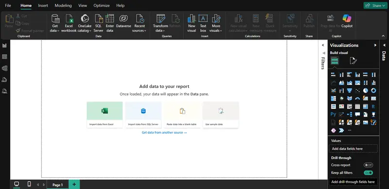
  2. Navigate to Home → Get Data → Excel
  3. Browse and select your Excel file
  4. In the Navigator window, select the required sheets or tables
  5. Click Load (to import directly) or Transform Data (to clean first)

Step 2: Connecting to Text/CSV Files

  1. Open Power BI Desktop
  2. Navigate to Home → Get Data → Text/CSV
  3. Browse and select the CSV file
  4. Preview the dataset in the dialog window
  5. Click Load or Transform Data

Step 3: Connecting to PDF

  1. Open Power BI Desktop
  2. Navigate to Home → Get Data → PDF → Connect
  3. Select the PDF file
  4. Wait for Power BI to detect available tables
  5. Select the desired table(s)
  6. Click Load or Transform Data

Step 4: Connecting to JSON

  1. Open Power BI Desktop
  2. Navigate to Home → Get Data → JSON
  3. Select the JSON file or input API endpoint
  4. Load the data into Power Query
  5. Expand nested fields to structure the data properly
  6. Click Close & Apply

Step 5: Connecting to SharePoint Folder

  1. Open Power BI Desktop
  2. Navigate to Home → Get Data → SharePoint Folder
  3. Enter the SharePoint site URL
  4. Click OK and authenticate if required
  5. Select files from the folder
  6. Click Combine & Transform Data

Step 6: Connecting to MySQL Database

  1. Open Power BI Desktop
  2. Navigate to Home → Get Data → More → Database → MySQL Database
  3. Enter the server name and database
  4. Provide authentication credentials
  5. Select the required tables
  6. Click Load or Transform Data

Step 7: Connecting to SQL Server

  1. Open Power BI Desktop
  2. Navigate to Home → Get Data → SQL Server
  3. Enter the server name (e.g., localhost)
  4. Leave the database field blank (or specify one if needed)
  5. Click OK
  6. Select authentication method (e.g., Windows credentials)
  7. In the Navigator pane, expand the database
  8. Select required tables
  9. Click Transform Data to open Power Query Editor

Step 8: Connecting to Web Data

  1. Open Power BI Desktop
  2. Navigate to Home → Get Data → Web
  3. Enter the URL of the web page or API
  4. Click OK
  5. Select the data table or structure detected
  6. Click Load or Transform Data

Step 9: Connecting to Azure Analysis Services

  1. Open Power BI Desktop
  2. Navigate to Home → Get Data → Azure → Azure Analysis Services
  3. Enter the server name
  4. Select the database/model
  5. Choose connection mode (Live connection recommended)
  6. Click Connect
    This structure improves readability, makes your blog actionable, and aligns well with real-world Power BI workflows.

Conclusion

Connecting to multiple data sources in Power BI is more than a technical process. It forms the foundation of every reliable and insight driven report. As highlighted, modern data environments are diverse and complex, requiring analysts to seamlessly work across files, databases, cloud services, and web platforms.

Power BI Desktop simplifies this complexity through its strong integration capabilities. When combined with Power Query, it enables not only data access but also a deeper understanding of data structure, quality, and limitations.

The true value, however, goes beyond simply connecting data. The ability to identify inconsistencies, manage missing values, and transform raw data into a clean and structured format is what distinguishes basic reporting from impactful analytics solutions.

In practice, effective data ingestion leads to

  • More accurate insights
  • Improved decision making
  • Scalable and maintainable data models.

As a Data professional, mastering data connectivity and preparation is essential. It ensures that every dashboard created is not only visually compelling but also reliable and meaningful.

Ultimately, great analytics begins with great data, and great data starts with how effectively it is connected, prepared, and understood.

pg-warehouse – A local-first data warehouse at scale without over Engineering that mirrors PostgreSQL data – no pipelines needed!

PostgreSQL → DuckDB → SQL Engine → Parquet →And beyond ….

A Local-First Analytics Pipeline

Data teams often spend more time operating infrastructure than actually building features.

To construct an AI feature pipeline, organizations frequently spin up heavy stacks consisting of:

Large cloud VMs
Distributed compute clusters
Streaming infrastructure
Data warehouses
Orchestration systems

These systems consume significant engineering effort and infrastructure cost before a single feature is produced.

The irony is that the core goal of most pipelines is simple: transform operational data into features for analytics or machine learning.

Yet the industry default architecture looks like this:

PostgreSQL → Kafka → Spark/Flink → Data Warehouse → Feature Store

This architecture is powerful — but also massively over-engineered for many workloads.

Most teams simply want to:

  • Mirror production data
  • Run SQL transformations
  • Generate datasets
  • Export them to analytics or AI pipelines

But instead they end up managing:

  • Kafka clusters
  • Spark jobs
  • Cloud warehouses
  • Orchestration systems
  • Infrastructure costs

For many workloads, this complexity isn’t necessary.

That observation led to the creation of pg-warehouse.

The Idea Behind pg-warehouse

pg-warehouse is a local-first pipeline engine that mirrors PostgreSQL OLTP data into a local DuckDB warehouse (analytical database).

It captures both:

  • The initial snapshot of tables
  • Incremental changes from PostgreSQL replication

Then developers can run SQL pipelines on top of the mirrored data.

The result:

PostgreSQL (OLTP)
      ↓
PostgreSQL replication stream
      ↓
pg-warehouse sync engine
      ↓
DuckDB local warehouse
      ↓
SQL feature pipelines
      ↓
Parquet / CSV datasets

Everything runs locally.

No Kafka.

No Spark.

No warehouse cluster.

Just:

PostgreSQL
DuckDB
SQL

Why PostgreSQL Replication?

Instead of polling tables or running ETL queries, pg-warehouse uses PostgreSQL’s native replication capabilities.

PostgreSQL exposes replication metadata through:

  • Write-Ahead Log (WAL)
  • Logical replication slots
  • LSN offsets

This allows pg-warehouse to:

  • Capture a consistent snapshot of selected tables
  • Track WAL changes after the snapshot
  • Apply incremental updates to DuckDB

This approach has several advantages:

  • minimal load on the OLTP database
  • exactly-once incremental progress
  • restart-safe replication

The sync engine tracks replication progress in a local state database.

Why DuckDB?

DuckDB is an ideal engine for local analytics workloads.

Key properties:

  • columnar storage
  • vectorized execution
  • high-performance SQL
  • embedded runtime

This allows pg-warehouse to transform row-oriented PostgreSQL data into *columnar analytics tables.
*

Example workflow:

SELECT
    user_id,
    COUNT(*) AS plays,
    MAX(created_at) AS last_activity
FROM raw.events
GROUP BY user_id

These pipelines generate derived feature tables that can be exported to Parquet.

Does its Scale?

What 90% of AI Data Pipelines Actually Do ..?

When people talk about PostgreSQL AI data pipelines, the architecture often looks intimidating:

PostgreSQL → SOME HEAVY DISTRIBUTED SYSTEMS → SOME EXPENSE CLOUD DATA WAREHOUSE → Feature Store → ML Pipeline

But if you examine the actual work performed inside most pipelines, the reality is much simpler.

Most pipelines are just SQL transformations. In practice, 90% of pipelines reduce to a few simple steps:

Typical Pipeline Operations

  • filter rows
  • aggregate events
  • join metadata
  • compute features

These are operations that columnar engines have optimized for decades. You don’t need a distributed compute cluster to do them.

Feature Tables Are Much Smaller Than Raw Data

Another reason pipelines are frequently over-engineered is a misunderstanding of how data volumes evolve across pipeline layers.

Raw event streams can be large, but feature tables are dramatically smaller.

If you ingest 200 GB of raw events per day, your final feature tables might only be 2–10 GB. That is well within the capabilities of a single-node columnar engine like DuckDB.

The 90% Pipeline Design Target

If you optimize a system for the following workload profile:

You can cover roughly 90% of real-world AI feature pipelines.
Everything beyond that tends to fall into hyperscale edge cases, such as:

  • trillion-event streaming systems
  • global ad-tech platforms
  • massive graph processing
  • real-time distributed ML training

These are important problems — but they are not the common case.

The Over-Engineering Problem

Modern data infrastructure often assumes that every pipeline must be built with distributed systems.

This leads to stacks like:

Kafka
Spark
Flink
Airflow
Data Warehouse
Feature Store

While powerful, these systems introduce significant overhead:

infrastructure complexity
operational cost
latency
specialized expertise

For many teams, this complexity is unnecessary.

A simpler architecture is often sufficient:

PostgreSQL
   ↓
DuckDB
   ↓
SQL feature pipelines
   ↓
Parquet datasets

Where pg-warehouse fits ?

pg-warehouse is designed specifically for this 90% case.

It mirrors PostgreSQL OLTP data into a local DuckDB warehouse, where developers can run SQL feature pipelines and export datasets to Parquet.

Instead of building complex distributed pipelines, developers can focus on the transformations that actually matter.

PostgreSQL
   ↓
Replication stream
   ↓
pg-warehouse
   ↓
DuckDB
   ↓
SQL feature pipelines
   ↓
Parquet datasets

The result is a local-first analytics stack that removes unnecessary infrastructure while still supporting the core transformations used in most AI pipelines.

Architecture

pg-warehouse is designed around a clean separation of concerns.

Open Core components include:

Sync Engine

Responsible for:

  • PostgreSQL snapshot
  • replication stream processing
  • applying changes to DuckDB

Warehouse Layer

DuckDB acts as the columnar analytics engine.

Tables are stored under the raw schema.

Pipeline Engine

Developers write SQL files describing feature pipelines.

Example:

pipelines/user_features.sql

These pipelines read from raw tables and produce derived datasets.

Export Engine

Exports datasets to:

  • Parquet
  • CSV
  • external storage

Design Principles

pg-warehouse follows several design constraints.

Local-First

The entire pipeline runs locally.

No cloud infrastructure required.

Single Binary

pg-warehouse is implemented in GoLang and compiled as a single executable.

This simplifies deployment dramatically.

Config-Driven

All workflows are configured using a single YAML file.

Example:

project:
  name: my_warehouse

postgres:
  url: postgres://warehouse:password@pg-host:5432/mydb
  schema: public

duckdb:
  raw: ./raw.duckdb
  silver: ./silver.duckdb
  feature: ./feature.duckdb

cdc:
  enabled: true
  publication_name: pgwh_pub
  slot_name: pgwh_slot
  tables:
    - public.orders
    - public.customers

sync:
  mode: incremental
  tables:
    - name: public.orders
      target_schema: raw
      primary_key: [id]
      watermark_column: updated_at
    - name: public.customers
      target_schema: raw
      primary_key: [id]
      watermark_column: updated_at

State Durability

Replication progress is stored in a SQLite state database.

This allows:

  • warehouse rebuilds
  • crash recovery
  • deterministic incremental sync

You can delete and rebuild your DuckDB warehouse without losing sync state.

Hexagonal Architecture

pg-warehouse follows a ports and adapters architecture.

Core logic is isolated from:

  • PostgreSQL adapter
  • DuckDB adapter
  • export adapters

This allows enterprise extensions without modifying core logic.

Open Core Model

pg-warehouse is an open core project.

Open Source includes:

  • PostgreSQL replication-based data sync
  • DuckDB local analytics warehouse
  • SQL feature pipelines
  • Parquet / CSV dataset export
  • Local-first pipeline execution

Enterprise features will include:

  • Cloud storage pipelines (S3 / GCS / Azure)
  • Version-controlled SQL pipelines
  • Distributed synchronization across nodes
  • Production observability and monitoring

Why This Matters

Data engineering is slowly shifting toward simpler architectures.

Modern embedded engines like DuckDB make it possible to run serious analytics workloads without clusters.

pg-warehouse aims to cover the 80% case for building datasets and AI features from PostgreSQL.

For many teams:

PostgreSQL → DuckDB → Parquet
Is enough.

Project

pg-warehouse is open core and available on GitHub.

Repository

Quick Start

Development Workflow

The Ultimate Guide: Installing Ollama on Fedora 43

Running large language models (LLMs) locally isn’t just for the privacy-obsessed anymore—it’s for anyone who wants a snappy, custom coding assistant without a monthly subscription. If you’re rocking Fedora 43, you’re already using one of the most cutting-edge distros out there.

Here is how to get Ollama up and running with full NVIDIA acceleration and hook it into VS Code for a seamless dev experience.

There’s something uniquely satisfying about seeing your GPU fans spin up because your local AI is thinking. Let’s get you there in eight steps.

Step 1: Open the Gates (RPM Fusion)

Fedora is known for its commitment to free, open-source software, which means the proprietary NVIDIA drivers aren’t there by default. We need to add the RPM Fusion repositories to get the “non-free” goodies.

Run this in your terminal:

$ sudo dnf5 install https://mirrors.rpmfusion.org/free/fedora/rpmfusion-free-release-$(rpm -E %fedora).noarch.rpm 

$ sudo dnf5 install https://mirrors.rpmfusion.org/nonfree/fedora/rpmfusion-nonfree-release-$(rpm -E %fedora).noarch.rpm

Note: We’re using dnf5 here, which is the faster, shinier version of the package manager standard in Fedora 43.

Step 2: The Driver Dance

Now, we install the NVIDIA drivers and the CUDA toolkit. This is what allows Ollama to talk to your GPU instead of making your CPU do all the heavy lifting.

sudo dnf5 install akmod-nvidia xorg-x11-drv-nvidia-cuda

A word of caution: Fedora moves fast. Sometimes, when the kernel updates, the NVIDIA modules need a moment to “catch up” (rebuild). If you update your system and things look wonky, it’s usually because the driver is still compiling in the background.

Step 3: The Classic Reboot

You know the drill. For the kernel to start using those new NVIDIA drivers, you need a fresh start. sudo reboot

Step 4: The Moment of Truth

Once you’re back in, let’s make sure Fedora and your GPU are on speaking terms. Run this command

nvidia-smi

If you see a table showing your GPU name and VRAM usage, congratulations—you’ve passed the hardest part.

Step 5: Installing Ollama

Ollama makes installation incredibly easy with a one-liner script. This script handles the heavy lifting: it downloads the binary, creates an ollama user/group, and sets up a systemd service so it starts automatically.

curl -fsSL https://ollama.com/install.sh | sh

Step 6: Verifying the GPU Link

Just because Ollama is installed doesn’t mean it’s using your GPU. It might be falling back to your CPU if it can’t find the drivers. Let’s check the logs:

journalctl -u ollama -b | grep "NVIDIA"

You’re looking for a line that confirms an NVIDIA GPU was detected. If you see it, you’re golden.

Step 7: Your First Local Run

Let’s test it with a lightweight, high-performance model. Qwen 2.5 Coder (0.5B version) is tiny but surprisingly “smart” for its size, making it perfect for a quick test.

ollama run qwen2.5-coder:0.5b

Once it downloads, you can chat with it directly in your terminal. Ask it to write a Python script; you’ll be impressed by the speed.

Integrating with VS Code (The “Continue” Extension)

Running AI in a terminal is cool, but having it inside your IDE is where the real productivity happens. We’ll use the Continue extension, which is an open-source powerhouse for local AI.

  • Install the Extension: Search for “Continue” in the VS Code Marketplace and install it.
  • Configure Local Access: Open the Continue sidebar, click the gear icon (settings), and select your local config file.
  • Edit the Config: Replace or add the following to your config.yaml (or config.json depending on your version) to point it toward your local Ollama instance:
name: Local Config
version: 1.0.0
schema: v1
models:
  - name: Qwen2.5-Coder 0.5B
    provider: ollama
    model: qwen2.5-coder:0.5b
    apiBase: http://localhost:11434
    roles:
      - chat
      - edit
      - apply
      - autocomplete
      - embed

Final Thoughts

You now have a fully private, incredibly fast AI coding assistant running on your local hardware. No data leaving your machine, no latency issues, and total control.

Regex: Tiny Pattern, Hidden Machine

https://www.youtube.com/watch?v=4xhxORnBeo4

You type a regex and it matches text. But under the hood, your regex engine is building and executing a full state machine — every single time.

From Pattern to Machine

A regex like a(b|c)*d looks simple. Five characters. But when the engine compiles it, here’s what actually happens:

  1. Each character becomes two states connected by a transition
  2. Concatenation chains state machines together
  3. Alternation (|) creates branching paths with epsilon transitions — free jumps that consume no input
  4. The star operator adds a loop from the accept state back to the start

This is Thompson’s construction, invented in 1968. Your tiny pattern becomes a nondeterministic finite automaton (NFA) — a graph with multiple possible paths at every step.

NFA → DFA: Removing the Guesswork

An NFA can be in multiple states at once. That’s powerful but expensive to simulate. So most engines convert it to a deterministic finite automaton (DFA) — one state at a time, one transition per input character.

The conversion uses the subset construction algorithm: each DFA state represents a set of NFA states. The trade-off? The DFA can have exponentially more states, but each step is O(1).

When Regex Goes Wrong

Not all engines use DFAs. Many (including Python, Java, JavaScript, Ruby, and PHP) use backtracking — they try one path, and if it fails, they back up and try another.

For most patterns, this is fine. But for patterns with nested quantifiers over overlapping characters, the number of paths explodes exponentially.

The pattern (a+)+b matched against aaaaaaaaaaX forces the engine to explore every possible way to divide those as into groups. Ten as? About a thousand paths. Twenty? Over a million. Thirty? Over a billion.

This is ReDoS — Regular Expression Denial of Service. One carefully crafted string can pin a CPU at 100% for hours.

Real incidents:

  • 2016: A regex crashed Cloudflare’s servers for 27 minutes
  • 2019: A single regex took down npm for 6 hours

The Fix

  • Avoid nested quantifiers over overlapping patterns
  • Use atomic groups or possessive quantifiers
  • Switch to an engine like RE2 that uses Thompson’s NFA simulation — linear time, guaranteed

Your regex is a program. And like any program, it can have performance bugs hiding in plain sight.

Watch the Full Video

The video walks through NFA construction, DFA conversion, backtracking simulation, and the ReDoS attack — all animated step by step.

References