Krafton, PUBG: Battlegrounds’un savaş alanlarını eğlenceye boğacak 1 Nisan etkinliği “Dekor Avı”nın bugün başladığını duyurdu. Dekor Avı modunda oyuncular iki role ayrılıyor. Avlar ve Avcılar. Avlar, haritaya dağılmış objelerin kılığına girerek gizleniyor; Avcılar ise alandaki şüpheli her şeyi arayarak süre dolmadan önce tüm obje kılığındaki Avları ortadan kaldırması gerekiyor. Bu oyun modu, gizlilik ve stratejiyi bir araya getirerek geleneksel savaş oyunlarının ötesinde yepyeni bir deneyim sunuyor. Her oyun toplamda 3 Avcı ve 9 Av olmak üzere 12 oyuncudan ve üç turdan oluşuyor. Her turun başında oyuncular tercih ettikleri rolü seçiyorlar; gerektiğinde takımlar otomatik olarak dengeleniyor. Oyun, birden fazla aşamadan oluşuyor. Hazırlık aşamasında, Avcılar kısıtlı bir alanda beklerken, Av rolündekiler kılık değiştirip saklanma yerlerini buluyor. Tur ilerledikçe, Avcılar obje kılığındaki Avları arayıp ortadan kaldırmaya başlıyorlar ancak oyuncu olmayan objelere ateş etmek Avcıların HP puanlarını düşürüyor. Bu nedenle alınan her karar beraberinde bir risk de taşıyor. Her turun sonuna doğru yaşanan kısa […]

PUBG: Battlegrounds’tan 1 Nisan’a özel “Dekor Avı” modu yazısı ilk olarak Teknoloji haberleri – LOG üzerinde yayınlandı.

In many applications, you don’t start with an address — you start with coordinates.

A user clicks on a map, shares their GPS location, or your system receives latitude and longitude from a device. But raw coordinates like 40.748817, -73.985428 aren’t very useful on their own. Most applications need human-readable data: a city name, a postal code, or a full address.

This is where reverse geocoding comes in.

In this article, we’ll look at how to convert latitude and longitude into structured address data — including city, postal code, and formatted address — and, more importantly, what developers should be aware of when working with real-world location data.

To make things more practical, we’ll also use a simple interactive demo where you can click on a map and instantly get the corresponding address details:

• CodePen Live Demo

Coordinates vs Address: Two Ways to Describe a Location

Latitude and longitude coordinates describe an exact point on Earth using a global grid system.

• latitude defines how far north or south a location is
• longitude defines how far east or west it is

Together, they pinpoint a precise location anywhere on the planet:

For example, the coordinates 40.748817, -73.985428 represent a specific point in New York.

However, while coordinates are extremely precise, they are not very intuitive for humans. People naturally think of locations in terms of:

• cities
• streets
• postal codes
• full addresses

This creates a gap between how machines represent locations and how humans understand them.

So how do you convert coordinates into a readable address?

To do that, you need a process that maps latitude and longitude to real-world location data — such as city names and postal codes. This process is called reverse geocoding.

Reverse Geocoding: Convert Coordinates to City, Postal Code, and Address

Reverse geocoding is the process of converting geographic coordinates (latitude and longitude) into a human-readable address.

In practice, reverse geocoding is not something you implement locally. It requires access to large, constantly updated geographic datasets that map coordinates to real-world address data — including administrative boundaries, streets, buildings, and postal codes.

Because of this, reverse geocoding is typically provided as a service via APIs.

One example is the Geoapify Reverse Geocoding API, which allows you to send coordinates and receive structured address data in response.

Here is an example API Request:

https://api.geoapify.com/v1/geocode/reverse?lat=40.748817&lon=-73.985428&format=json&apiKey=YOUR_API_KEY

The response contains structured fields such as:

• city, town, village
• postcode
• street, housenumber
• formatted (full address)

You can also control the level of detail using the type parameter, which helps filter results by address level (for example: city, postcode, street, etc.).

Getting city from coordinates

To get the city from coordinates, you can use reverse geocoding with the type=city parameter. This tells the API to return results at the city level.

For example:

https://api.geoapify.com/v1/geocode/reverse?lat=40.719726903683636&lon=-74.04103305850015&format=json&type=city&apiKey=YOUR_API_KEY

A typical response looks like this:

{
  "results": [
    {
      "country": "United States",
      "state": "New Jersey",
      "city": "Jersey City",
      "lon": -74.047455,
      "lat": 40.7215682,
      "result_type": "city",
      "formatted": "Jersey City, NJ, United States of America",
      "address_line1": "Jersey City, NJ",
      "address_line2": "United States of America",
      ...
    }
  ]
}

Using type=city ensures that the response focuses on the city-level administrative area, rather than returning street-level or building-level details.

Getting postcode (ZIP code) from coordinates

To get the postal code from coordinates, you can use reverse geocoding with the type=postcode parameter. This ensures the API returns results at the postcode level.

For example:

https://api.geoapify.com/v1/geocode/reverse?lat=40.739501996228256&lon=-74.18542863164123&type=postcode&format=json&apiKey=YOUR_API_KEY

A typical response looks like this:

{
  "results": [
    {
      "country": "United States",
      "state": "New Jersey",
      "city": "Newark",
      "postcode": "07103",
      "result_type": "postcode",
      "formatted": "Newark, NJ 07103, United States of America",
      "address_line1": "Newark, NJ 07103",
      "address_line2": "United States of America"
    }
  ]
}

The key field here is:

• postcode — contains the postal (ZIP) code for the given coordinates

Additional useful fields include:

• city — the associated city
• formatted — full human-readable address

Using type=postcode ensures that the response focuses specifically on postcode-level data.

Keep in mind that:

• not all locations have postal codes
• postal codes may represent areas rather than exact points
• formats vary depending on the country

Getting address from coordinates

To get a full address from coordinates, you can use reverse geocoding without specifying a type, which returns the most relevant place for the given location (for example, a building, POI, or street address).

For example:

https://api.geoapify.com/v1/geocode/reverse?lat=40.68818115914695&lon=-73.99558678565592&format=json&apiKey=YOUR_API_KEY

A typical response looks like this:

{
  "results": [
    {
      "name": "Citi Bike - Congress St & Clinton St",
      "housenumber": "183",
      "street": "Congress Street",
      "city": "New York",
      "postcode": "11201",
      "state": "New York",
      "country": "United States",
      "result_type": "amenity",
      "formatted": "Citi Bike - Congress St & Clinton St, 183 Congress Street, New York, NY 11201, United States of America",
      "address_line1": "Citi Bike - Congress St & Clinton St",
      "address_line2": "183 Congress Street, New York, NY 11201, United States of America"
    }
  ]
}

The most useful field for display is:

• formatted — a ready-to-use human-readable address

You can also access individual components such as:

• name — place or POI name (if available)
• housenumber and street
• city, postcode, state, country

By default, reverse geocoding returns the most relevant result for the given coordinates, which may be a specific place (like a business or landmark), not just a street or city.

Common Pitfalls When Converting Coordinates to Address

Reverse geocoding is powerful, but working with real-world location data comes with a few important caveats.

Understanding these will help you avoid common mistakes and build more reliable applications.

City is not always available

Not every location has a city field. Depending on where the coordinates point, the response may include:

• city
• town
• village
• or no settlement at all

To handle this correctly, always implement a fallback strategy instead of relying on a single field.

The result depends on the exact point

Small changes in coordinates can lead to different results.

For example, clicking on:

• a building → returns a specific address
• a road → returns street-level data
• a park → may return only city or district

This is expected behavior, not an error.

The closest result may not match expectations

Reverse geocoding returns the nearest known object.

This could be:

• a building
• a business (POI)
• a street
• an administrative area

If you need a specific level (e.g., city or postcode), use the type parameter to control the result.

Coordinates may need normalization

Coordinates should always be valid:

• latitude must be between -90 and 90
• longitude must be between -180 and 180

Try It Yourself: Interactive Reverse Geocoding Demo

To better understand how reverse geocoding works in practice, try this interactive demo:

Live Demo on CodePen

The demo also shows how different clicks can return different types of results depending on the location — for example, a building, a street, or an administrative area.

Summary

Converting latitude and longitude into a city, postal code, or full address is a common requirement in many applications — from delivery services to map-based interfaces.

In this article, we explored how reverse geocoding works and how to use it to extract meaningful location data from coordinates.

Key takeaways:

• coordinates describe precise locations, but are not human-friendly
• reverse geocoding bridges the gap between coordinates and real-world addresses
• you can extract specific data like city and postcode using the type parameter
• not all locations have complete address data, so fallback logic is important
• results may vary depending on the exact coordinates and context

By understanding these concepts and handling edge cases properly, you can build reliable features that convert coordinates into usable address information.

Additional Resources

• Geoapify Reverse Geocoding API
• MapLibre GL JS Documentation
• Live Demo on CodePen

FAQ

Is reverse geocoding free?

Most reverse geocoding services offer a free tier with usage limits.

For example, Geoapify provides a free plan with 3000 requests per day and 5RPS. This is usually enough for testing and small applications. For production use or higher volumes, paid plans are available.

How do I get an API key?

To use a reverse geocoding service like Geoapify, you need an API key.

You can get one by registering at the website.

After creating a project, you’ll receive an API key that you can use in your requests.

How do I get the timezone from coordinates?

Reverse geocoding responses often include timezone information.

For example, Geoapify returns a timezone object with:

{
  "name": "America/New_York",
  "offset_STD": "-05:00",
  "offset_STD_seconds": -18000,
  "offset_DST": "-04:00",
  "offset_DST_seconds": -14400,
  "abbreviation_STD": "EST",
  "abbreviation_DST": "EDT"
}

You can extract this directly from the response without making a separate API call.

How do I get the state or region?

To get the state or region from coordinates, you can use reverse geocoding with the type=state parameter. This ensures the API returns results at the state level.

How can I understand the quality of the result?

You can estimate how accurate the result is using the distance field.

• distance represents how far (in meters) the returned result is from the input coordinates
• smaller values indicate higher accuracy

For example:

• 0–10 meters → very precise (building-level)
• 10–100 meters → good accuracy
• 100+ meters → approximate result

Why do I sometimes get a place (POI) instead of an address?

By default, reverse geocoding returns the most relevant nearby object.

This could be:

• a business or landmark (POI)
• a building
• a street
• an administrative area

If you need a specific level (e.g., city or postcode), use the type parameter to control the result.

Can I use reverse geocoding offline?

In most cases, no.

Reverse geocoding requires large and frequently updated datasets, making it impractical to run locally. That’s why it is typically provided as an online API service.

What happens if there are no results?

In some cases, reverse geocoding may return no results:

• remote areas
• oceans or lakes
• incomplete data coverage

Your application should handle this gracefully and provide fallback behavior.

The bill arrives before the alert does. Because the system that creates the cost isn’t the system you’re monitoring.

Inference observability isn’t a tooling problem — it’s a layer problem. Your APM stack tracks latency. Your infrastructure monitoring tracks GPU utilization. Neither one tracks the routing decision that sent a thousand requests to your most expensive model, or the prompt length drift that silently doubled your token consumption over three weeks.

By the time your cost alert fires, the tokens are already spent.

The Visibility Gap

Inference cost is generated at the decision layer. Routing decisions, token consumption, model selection, retry behavior — these are the variables that determine what you pay. But most observability exists at the infrastructure layer.

Here’s how the layers break down:

The inference layer is where routing decisions get made, where token budgets get consumed, where cache hits and misses determine whether you’re paying for compute or serving from memory. It’s also the layer that most monitoring stacks treat as a black box.

The 5 Signals That Predict Cost Before It Spikes

Standard metrics tell you what happened. These signals tell you what’s about to happen.

Signal 01 — Token Consumption Rate (spend velocity)
Tokens per second per endpoint. A spike in token consumption rate precedes a cost spike by minutes to hours. Track it at the endpoint level, not the aggregate.

Signal 02 — Prompt Length Drift (silent cost multiplier)
The p95 prompt length over time. When prompt length drifts upward — users adding more context, system prompts growing, retrieval chunks increasing — token cost grows with it. No alert fires. No system breaks. The bill just quietly doubles over three weeks.

Signal 03 — Cache Hit Rate (efficiency signal)
Semantic cache and KV cache hit rates. A cache hit rate drop from 40% to 20% doubles your effective inference cost with no change in request volume. Most teams don’t instrument it at all.

Signal 04 — Routing Distribution (decision quality signal)
The percentage of requests hitting each model tier. When routing distribution drifts — more requests hitting your frontier model than expected — cost escalates without any system error.

Signal 05 — Retry Rate (failure cost amplifier)
Failed requests that retry still consume tokens on the failed attempt. A 10% retry rate means 10% of your token spend generated zero value.

What to Instrument — The 3-Layer Observability Stack

Instrumentation must exist at the same layer where decisions are made.

Decision Layer (request-level)

• Tokens in / tokens out per request
• Model selected
• Routing path taken
• Cost per request
• Cache hit or miss
• Latency to first token

Behavior Layer (session-level)

• Total token budget consumed per session
• Routing path distribution
• Retry count
• Prompt length trend
• Token budget remaining vs elapsed session time

Business Layer (aggregate)

• Cost per feature
• Cost per user cohort
• Token burn rate (velocity)
• Routing distribution drift
• Cache efficiency trend
• Budget utilization rate

The Budget Signal Pattern

Dollar alerts are lagging indicators. Token rate alerts are leading indicators.

Most teams set cost alerts at the dollar level. By the time that alert fires, the tokens are already spent, the requests already executed, the routing decisions already made. You can’t stop a cost spike that already executed.

Token rate — tokens consumed per minute per endpoint — fires earlier. A token rate anomaly is detectable within minutes of a routing change, a prompt length drift, or a cache configuration failure.

Where Inference Observability Fails

Most teams can tell you what they spent. Very few can tell you why.

[01] Tracking latency, not tokens.
Response time is green. Token consumption has been climbing for two weeks. The system looks healthy. The bill doesn’t.

[02] Tracking errors, not retries.
Error rate is 0.1%. Retry rate is 12%. Every retry is a token burn that generated zero output value.

[03] Tracking requests, not routing paths.
Request volume is flat. Routing distribution has drifted — 60% of requests now hitting the frontier model instead of the expected 20%. Volume didn’t change. Cost per request tripled.

[04] Tracking cost, not cause.
Monthly spend alert fires. The investigation begins after the fact — sifting through logs to reconstruct which routing decision, which prompt length drift, which cache failure caused it. Post-incident analysis, not prevention.

How the Series Connects

This series has been building a single architecture across four posts:

• Part 1 — The cost model: why inference behaves like egress
• Part 2 — Execution budgets: runtime controls that cap spend before it cliffs
• Part 3 — Cost-aware routing: getting requests to the right model at the right cost
• Part 4 — Observability: the feedback loop that makes the other three work

Without observability, the other three are blind. Budgets are unvalidated. Routing is unconfirmed. Cost model predictions are theoretical.

Architect’s Verdict

You can’t enforce a budget you can’t see. And you can’t see inference cost until you instrument the decision layer.

Instrument the decision layer. Set token rate alerts, not just dollar alerts. Track routing distribution as a cost signal. Treat cache hit rate as an efficiency metric with direct cost implications.

The goal isn’t more dashboards — it’s visibility at the layer where cost decisions are actually made. That’s the only layer where intervention is still possible.

Full post with HTML diagrams, the visibility gap table, and the complete 5-signal card breakdown: rack2cloud.com/ai-inference-observability

Part of the AI Infrastructure Architecture series on Rack2Cloud.

tl;dr: We reduced Google Kubernetes Engine(GKE) costs by 60%. The biggest wins came not from Kubernetes tuning, but from understanding why our Rails app needed so many Pods in the first place:

• Rails was running 1 Puma worker with 33 threads. Ruby’s GVL made this effectively single-core. We switched to 4 workers with 8 threads.
• API authentication used bcrypt on every request. We replaced it with a lighter method.
• GKE node generation was outdated: upgrading from n1 to n2d gave 56% more CPU, 23% more RAM, for 3% less cost.
• Only after fixing per-Pod efficiency did we add KEDA Cron autoscaling and GKE node autoscaling.

The order mattered. We improved per-Pod efficiency first, then used autoscaling to stop paying for idle capacity. The interesting part was not any one change by itself, but why these four changes reinforced each other. The rest of this article walks through the reasoning behind each one.

I work on a B2B SaaS platform that runs on Google Kubernetes Engine. The API server is a Rails application, and it was the biggest cost driver on our GKE cluster.

Over the course of about nine months, we reduced GKE costs by roughly 60%, with most of the core technical changes concentrated in July and August 2025. Most of the savings came from understanding how Rails actually uses CPU and memory, and fixing misconfigurations that had been in place since launch. The Kubernetes-level changes (autoscaling, node upgrades) were important, but they only worked well because we fixed the application layer first.

The key was looking at the system holistically, from Ruby’s runtime behavior to Kubernetes scaling. This article explains why the savings came from four changes applied in the right order: better GKE node price-performance, a Rails process model that matched Ruby’s concurrency model, removing unnecessary per-request CPU work, and only then introducing autoscaling.

The vicious cycle: why the cluster needed so many Pods

The high cost was not caused by a single problem. It was a cycle:

1. Inefficiency: Rails performance was poor, partly due to misconfigured concurrency settings and a CPU-heavy authentication path.
2. Over-provisioning: To handle traffic, we compensated by running more Pods.
3. Waste: There was no autoscaling, so those Pods ran 24/7 regardless of actual demand.
4. High Unit Cost: The nodes were old-generation instances with worse price-performance.

Each problem amplified the others. Inefficient Pods meant we needed more of them, which meant more nodes to host them, all running around the clock.

The reduction did not come from one dramatic optimization. It came from breaking this cycle at multiple points: making each Pod more efficient, reducing unnecessary CPU work, and only then allowing the cluster to scale with demand.

How the cost actually came down

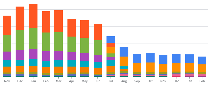
Before diving into the technical details, here is what the cost trajectory looked like. The chart below shows monthly GKE spending by SKU. The trend is clear.

This was not primarily a traffic reduction. API traffic remained broadly stable during this period, and the savings came mainly from efficiency improvements.

The reduction happened in two phases.

In the first phase (early 2025 through June 2025), we simply reduced Pod and node counts that were clearly excessive. This brought costs down from the peak, but it was just trimming fat. The underlying inefficiencies remained.

The second phase (July 2025 onward) is where the real optimization happened. It breaks down into two parts:

• Part 1: Static optimization — making each Pod and each node as efficient as possible.
• Part 2: Dynamic optimization — scaling capacity up and down with demand.

Part 1: Static Optimization

1.1 GKE Node generation upgrade: n1-highmem-2 → n2d-highmem-2

Our GKE nodes had been running on n1-highmem-2 since the early days of the service. The n1 family is Google Cloud’s first generation of general-purpose instances, based on older Intel Skylake/Broadwell processors.

We migrated to n2d-highmem-2, which uses AMD EPYC processors. The performance difference is significant. According to Google’s official CoreMark benchmarks:

56% more CPU performance. 23% more RAM. 3% lower cost. The newer generation is faster, has more memory, and is cheaper.

For us, this was one of the rare optimizations that improved both performance and cost at the same time. The migration itself was straightforward: update the node pool configuration, cordon and drain the old nodes, and let the new pool take over. We did this in July 2025, and it shows up as a clear inflection point in the billing data.

This time, we chose x86-based N2D rather than Arm to preserve binary compatibility and minimize ecosystem risk around Ruby, native extensions, and container images. It was the most practical low-risk step. That said, Arm remains a possible next step for further cost reduction.

If your GKE nodes are still running on n1-series instances, check the benchmarks and pricing for n2d or newer.

1.2 Rails process model: from 33 threads to 4 workers

This was probably the biggest single contributor to the cost reduction.

Our Rails application was running Puma with the following configuration:

• WEB_CONCURRENCY was not set (defaults to 1, meaning a single worker process)
• RAILS_MAX_THREADS=33

So we had one process with 33 threads. On the surface, that sounds like it should handle 33 concurrent requests efficiently. In practice, it did not give us the kind of throughput we expected, because of how Ruby works.

Ruby’s Global VM Lock (GVL)

Ruby has a Global VM Lock (GVL). Only one thread can execute Ruby code at a time within a single process. Multiple threads help when threads are waiting on I/O (database queries, HTTP calls, file reads), because a waiting thread releases the GVL and lets another thread run. But for CPU-bound work, 33 threads in one process gives you essentially the same CPU throughput as 1 thread.

This meant our 33-thread setup was an illusion. We were paying for the memory overhead of 33 thread stacks without getting the CPU parallelism we thought we had.

The bcrypt problem

On top of the GVL issue, our API used bcrypt for token authentication on every request. bcrypt is designed to be slow. That is its purpose as a password hashing algorithm: it is intentionally CPU-intensive to make brute-force attacks impractical.

But we were running bcrypt on every API call, not just on login. Modern versions of bcrypt-ruby release the GVL during computation, so it does not block other threads. However, the CPU cost itself remains significant. Every API request was burning CPU cycles on an expensive hashing operation, eating into the Pod’s overall processing capacity. With hundreds of API calls per minute, this added up.

We replaced bcrypt with a lighter authentication method for API token validation. The specifics of the new approach are not relevant here, but the key point is: bcrypt is the right tool for password hashing at login. It is the wrong tool for per-request API authentication.

The fix

We changed the Puma configuration to:

• WEB_CONCURRENCY=4 (4 worker processes)
• RAILS_MAX_THREADS=8

Four worker processes, each with its own GVL, running on separate CPU cores. This gives actual CPU parallelism. Thread count was reduced to 8 per worker, which is enough for I/O concurrency without the memory overhead of 33 threads. That said, 8 is still conservative. Since Rails 7.2, the default Puma thread count is 3 per worker, reduced from the previous default of 5. We may reduce this further in the future, which would lower per-worker memory consumption even more. For guidance on tuning worker and thread counts for your environment, see Puma’s deployment documentation.

The memory impact was counterintuitive. You might expect 4 workers to use 4x the memory of 1 worker. They do not, thanks to Copy-on-Write (CoW). When Puma forks worker processes, the child processes share the parent’s memory pages. They only allocate new memory when they write to a page. In practice, a large portion of the Rails application code, gems, and boot-time data remains shared.
One important requirement for this to work is to use preload_app! in your Puma configuration. Without it, each worker loads the application independently after forking, and memory sharing does not happen.

We also set the environment variable MALLOC_ARENA_MAX=2 to reduce glibc’s memory arena overhead. You can think of it as a small but useful guardrail against glibc holding on to too much memory. By default, glibc creates up to 8 * CPU cores malloc arenas, each of which holds onto freed memory independently. In a multi-process Rails setup, this leads to significant memory waste. Setting MALLOC_ARENA_MAX=2 cut per-Pod memory consumption by roughly 20%. I wrote a more detailed article about this:

Why Rails App Memory Bloat Happens: Causes and Solutions (and How I Cut It by 20%)

Katz Sakai

Katz Sakai

Katz Sakai

Follow

Mar 26

Why Rails App Memory Bloat Happens: Causes and Solutions (and How I Cut It by 20%)

#ruby
#rails
#performance
#linux

25 reactions

Comments

Add Comment

5 min read

Between CoW, MALLOC_ARENA_MAX, and fewer threads, our Pod memory request actually decreased from 4.2Gi to 3.5Gi, even after moving from one worker process to four.

That means the memory cost of achieving real CPU parallelism dropped significantly.

But the memory improvement was secondary. The real cost impact was the reduction in Pod count. Previously, each Pod had only one Puma worker, which limited CPU-parallel Ruby execution and forced us to run more Pods to handle traffic. With 4 workers per Pod, the same traffic can be served by far fewer Pods. Fewer Pods means fewer nodes, and that is where the cost savings came from.

Part 2: Dynamic Optimization

With each Pod running more efficiently, the next step was to stop paying for capacity we did not need outside of peak hours. But before turning on autoscaling, we needed to make sure Pods could be safely started and stopped at any time.

2.0 Prerequisites: making Pods safe to autoscale

Autoscaling means Kubernetes is constantly creating and destroying Pods. If your Pods are not set up for this, you trade cost savings for reliability problems.

We configured the following before enabling any autoscaling:

Startup probe. Our Rails application takes a while to boot. It loads the framework, initializes gems, establishes database connections, and warms up caches. Without a startup probe, Kubernetes may decide the Pod is unhealthy and kill it before it finishes starting. The startup probe gives the Pod the time it needs to complete initialization before liveness checks begin.

Readiness probe. This tells Kubernetes whether a Pod is ready to accept traffic. If a Pod becomes temporarily unable to serve requests (for example, during a heavy background job or a lost database connection), the readiness probe fails and the Pod is removed from the Service’s endpoints until it recovers.

Liveness probe. This detects Pods that are running but stuck (a hung Rails process, for example). Kubernetes automatically restarts them. This is important for long-running Pods.

terminationGracePeriodSeconds. When KEDA scales in Pods during the evening, in-flight requests need time to complete. The grace period tells Kubernetes to wait before forcefully killing the Pod, preventing dropped requests during scale-in. In practice, setting the grace period alone may not be enough. Kubernetes removes the Pod from the Service endpoints in parallel with sending the termination signal, so some requests can still arrive after shutdown begins. Adding a short preStop hook (e.g., sleep for a few seconds) gives the endpoints update time to propagate. See this article on graceful Kubernetes deployments for a detailed explanation of the timing issue.

These are not optional extras. They are prerequisites. Without them, autoscaling works on paper but fails in production. For details on configuring each probe type, see the Kubernetes documentation on liveness, readiness, and startup probes.

2.1 KEDA with Cron trigger

Before KEDA, our Pods ran at peak capacity 24/7. The replica count was set to handle the busiest time of day, and it stayed there overnight, on weekends, and on holidays.

Our platform is a business application. Usage concentrates on weekday business hours (roughly 8:30 to 19:30 JST). Evenings and weekends are quiet. This traffic pattern is stable and predictable.

Given this predictability, we chose KEDA‘s Cron trigger. KEDA is an event-driven autoscaler for Kubernetes, and the Cron trigger is one of its simplest scaling options: it adjusts the replica count on a time-based schedule, rather than reacting to metrics like CPU or memory usage. When you know the traffic pattern in advance, this is simpler and more reliable than reactive scaling. There is no lag waiting for metrics to cross a threshold, no risk of flapping, and the configuration is easy to understand.

Our configuration:

• Weekdays 08:00-20:00 JST: about 3–4x more replicas than the baseline off-hours level
• All other times: baseline replica count

No metrics, no thresholds, no reactive logic. For our traffic pattern, that simplicity was a feature, not a limitation.

One thing to note: Cron-based scaling assumes the traffic pattern stays stable. As the business grows, the current replica counts may not be enough. To catch this early, we monitor API response times with external synthetic monitoring. If response times start creeping up during business hours, that is the signal to revisit the replica counts. Cron scaling is not set-and-forget. It just changes infrequently.

2.2 GKE Node Autoscaling

With Pod counts now fluctuating on KEDA’s schedule, we enabled GKE’s Cluster Autoscaler.

The logic is straightforward: when KEDA scales Pods down in the evening, some nodes end up underutilized. The Cluster Autoscaler drains those nodes and removes them. When KEDA scales Pods back up in the morning, the autoscaler provisions new nodes to accommodate them. We configured a minimum node count for availability zone redundancy and a maximum to cap costs.

The combination of KEDA controlling Pod count and the Cluster Autoscaler controlling node count means we only pay for the capacity we are actually using.

Results

Comparing the H2 2024 average (before optimization) to the Q1 2026 average (after all changes were in place):

The cost declined steadily from February 2025 through September 2025 as each optimization was rolled out. The N1 to N2D node migration in July 2025 is visible as a clear step down in the billing data. Costs stabilized from late 2025 onward.

Lessons learned

None of these were particularly glamorous optimizations. Most were the kind of changes teams postpone because each one seems too small to matter. But together, they changed the economics of the entire system.

The ordering mattered as much as the individual changes. The biggest lesson was that cost optimization is not primarily about scaling policies. It is about unit economics. First make each Pod cheaper and more productive. Then let autoscaling amplify that efficiency. If we had introduced autoscaling first, we would simply have scaled an inefficient system up and down. The real savings only appeared after we improved per-Pod efficiency.

Understand your runtime’s concurrency model. Ruby’s GVL means threads do not give you CPU parallelism. If your Rails app has a high thread count and a single Puma worker, you are paying for memory without getting the concurrency you expect. Use multiple workers for CPU parallelism, and set thread count based on I/O concurrency needs only.

bcrypt is for passwords, not for API tokens. bcrypt is intentionally slow. Running it on every API request is a CPU tax that adds up quickly. Use it where it belongs (password hashing at login) and use something lighter for per-request token validation.

Boring autoscaling is good autoscaling. KEDA supports dozens of trigger types, including metrics-based, queue-based, and custom triggers. But for a business application with a predictable traffic pattern, a Cron trigger is the right choice. Do not build complexity you do not need.

Review your resource allocations regularly. If your Pod requests and limits have not changed since the service launched, they are almost certainly wrong. Workloads evolve, but resource specifications tend to stay frozen.

Node generations matter more than you think. Upgrading from n1 to n2d gave us 56% more CPU, 23% more RAM, and 3% lower cost. The migration effort was minimal. If you are still on n1, just do it.

Looking back, the 60% cost reduction came from being willing to look across the full stack, from Ruby’s runtime model to Kubernetes scaling policies, rather than optimizing within a single layer.

For more on the Rails memory topic, see my article:

Why Rails App Memory Bloat Happens: Causes and Solutions (and How I Cut It by 20%)

Katz Sakai

Katz Sakai

Katz Sakai

Follow

Mar 26

Why Rails App Memory Bloat Happens: Causes and Solutions (and How I Cut It by 20%)

#ruby
#rails
#performance
#linux

25 reactions

Comments

Add Comment

5 min read