AitherOS vs AutoGen: Which Multi-Agent Framework Should You Use in 2026?

AitherOS vs AutoGen: Which Multi-Agent Framework Should You Use in 2026?

In 2026, the choice between AitherOS and AutoGen for multi-agent AI orchestration depends primarily on your deployment requirements and workflow complexity. AitherOS excels for teams needing a complete self-hosted system with a UI, real-time visibility, human-in-the-loop controls, and built-in Kanban workflows. AutoGen is better for Python developers integrating agent capabilities into existing codebases or requiring maximum API flexibility. This article provides an in-depth comparison to help you choose the right framework for your specific needs.

Architecture Comparison: AutoGen vs AitherOS

Both frameworks enable multi-agent coordination, but their architectural approaches differ significantly. Here’s how they compare across key dimensions:

Feature AitherOS AutoGen
Core Architecture Full-stack system (Go backend, Next.js UI, PostgreSQL, Redis) Python library (Core API, AgentChat API, Extensions)
Self-hosted web UI ✅ Real-time dashboard ❌ (AutoGen Studio is a prototype tool)
Execution visibility ✅ Live stream of agent messages, tool calls, status ❌ Log files only
Tool layer ✅ Built-in MCP server with 50+ tools ✅ MCP support via extensions
Long-term memory ✅ Per-workforce vector knowledge base (pgvector) ❌ (requires custom implementation)
Human-in-the-loop ✅ Intervention, halt/resume, strategy approval ✅ Via human proxy agent
Credential management ✅ Encrypted vault per workforce ❌ (environment variables)
Kanban/task tracking ✅ Built-in with autonomous scheduling ❌ (requires external tools)
Native image generation ✅ Integrated with multiple providers ❌ (requires extensions)
Multi-provider support ✅ Mix models within one workflow ✅ Via model clients
Programming language Go backend, JavaScript frontend Python (+ .NET support)
License AGPL (commercial licenses available) MIT

Key Architectural Differences

AitherOS: Designed as a complete system where agents, tools, memory, and coordination layers run together as a unified service. It’s built for teams who need a production-ready platform rather than a library to integrate into existing code. The Go backend handles orchestration, the Next.js frontend provides real-time visibility, PostgreSQL with pgvector enables knowledge storage, and Redis powers the event bus.

┌─────────────────────────────────────────────────────────────┐
│                     Browser / Operator                       │
│              Next.js 16 · React 19 · WebSocket              │
└──────────────────────────┬──────────────────────────────────┘
                           │ HTTPS + WSS
┌──────────────────────────▼──────────────────────────────────┐
│                    AitherOS Backend (Go)                     │
│                                                             │
│  ┌──────────────────┐  ┌────────────────┐  ┌─────────────┐ │
│  │   Orchestrator   │  │   Event Bus    │  │  Knowledge  │ │
│  │                  │  │                │  │    (RAG)    │ │
│  │  Planning        │  │  Redis pub/sub │  │             │ │
│  │  Discussion      │  │  + in-process  │  │  pgvector   │ │
│  │  Exec rounds     │  │  channels      │  │  cosine sim │ │
│  │  Peer consult    │  │                │  │  auto-embed │ │
│  │  Synthesis       │  └────────────────┘  └─────────────┘ │
│  │  QA review       │                                       │
│  │  Auto scheduler  │  ┌────────────────┐  ┌─────────────┐ │
│  └──────┬───────────┘  │  MCP Manager   │  │  Provider   │ │
│         │              │                │  │  Registry   │ │
│         │              │  stdio/SSE     │  │             │ │
│         │              │  session pool  │  │  LLM/embed/ │ │
│         │              │  tool dispatch │  │  image/audio│ │
│         │              └────────────────┘  └─────────────┘ │
└─────────┼───────────────────┬─────────────────────────────┘

AutoGen: Built as a modular Python library with a layered architecture. It provides Core API (message passing, event-driven agents), AgentChat API (high-level chat patterns), and Extensions API (model clients, tools). This design prioritizes flexibility and integration into existing Python workflows rather than providing a standalone system.

import asyncio
from autogen_agentchat.agents import AssistantAgent
from autogen_agentchat.tools import AgentTool
from autogen_ext.models.openai import OpenAIChatCompletionClient

# Example of AutoGen's modular architecture
async def main() -> None:
    model_client = OpenAIChatCompletionClient(model="gpt-4.1")

    # Create specialist agents
    math_agent = AssistantAgent(
        "math_expert",
        model_client=model_client,
        system_message="You are a math expert.",
    )

    # Create agent tools for orchestration
    math_agent_tool = AgentTool(math_agent)

    # Main agent that orchestrates
    agent = AssistantAgent(
        "assistant",
        system_message="You are a general assistant. Use expert tools when needed.",
        model_client=model_client,
        tools=[math_agent_tool],
        max_tool_iterations=10,
    )

When to Choose AutoGen

AutoGen is the better choice when:

  1. You need Python library integration: Your existing codebase is Python-based, and you want to integrate multi-agent capabilities directly into your application rather than running a separate service.
  2. Maximum API flexibility is required: You need fine-grained control over agent implementation, message routing, and customization at the code level.
  3. Development environment focus: You’re primarily building prototypes or research projects where a UI and persistence layer aren’t essential.
  4. Minimal deployment complexity: You prefer to avoid setting up and maintaining a full-stack system with databases and separate services.
  5. License requirements: Your organization requires MIT-licensed components, especially for embedding into commercial products without open-sourcing your code.

Example AutoGen use case: A research team building a custom AI research assistant that will be integrated into their existing Python data science platform, where having code-level control over agent behavior is more important than UI visibility.

When to Choose AitherOS

AitherOS is the better choice when:

  1. You need a complete system: You want a production-ready platform rather than a library to integrate—including UI, database, tools, and orchestration in a unified system.
  2. Real-time visibility matters: Your teams need to see agent activity, tool usage, and execution status in real time through a web dashboard.
  3. Human-in-the-loop workflows: Your use cases require supervisory control, intervention capabilities, and the ability to halt or resume executions mid-stream.
  4. Long-term memory requirements: You need built-in vector storage to accumulate knowledge across multiple executions and provide context to future agent runs.
  5. Kanban-style task management: You want a structured approach to task tracking, autonomous scheduling, and QA review of agent outputs.
  6. Credential management: Security concerns require proper encryption and isolation of API keys and credentials between different agent teams.

Example AitherOS use case: A software development team running autonomous coding agents that require persistent workspaces, credential management for multiple APIs, a Kanban board for feature tracking, and a human approver to review generated code before it’s committed.

Execution Lifecycle Comparison

The execution models highlight key philosophical differences between the frameworks:

AitherOS Execution Lifecycle

Objective
    │
    ▼
[Planning]          leader agent decomposes into per-agent subtasks
    │
    ▼
[Discussion]        agents debate approach, reach consensus strategy
    │               
    ▼
  Human approves strategy  ──► (or auto-approved)
    │
    ▼
[Execution Rounds]  coordinated round-robin subtask execution
    │    └──────────► [Peer Consultation]  agent asks peer mid-task
    │                                      peer responds, agent continues
    ▼
[Synthesis]         leader assembles final output from all subtask results
    │
    ▼
[QA Review]         LLM checks output against kanban task acceptance criteria
    │               passed → Done  /  flagged → Blocked for human review
    ▼
[Knowledge Ingest]  execution result + messages embedded into vector KB

AitherOS follows a structured, phase-based approach with explicit planning, discussion, execution, synthesis, QA, and knowledge ingestion phases. This formalized process ensures comprehensive task breakdown and quality control.

AutoGen Execution Approach

AutoGen provides flexible patterns rather than a single workflow, with common patterns including:

  1. Assistant-Human Chat: Simple back-and-forth between an assistant agent and a human proxy.
  2. Two-Agent Chat: Automated conversation between two specialized agents, such as a user proxy and an assistant.
  3. Group Chat: Multiple agents participating in a shared conversation, with optional human involvement.
  4. Tool-Using Agent: A single agent leveraging tools through function-calling APIs.
  5. Agent Orchestration: Using AgentTool to coordinate multiple specialist agents.

This flexibility allows developers to implement custom patterns but requires more code to achieve structured workflows like AitherOS’s built-in execution lifecycle.

Migration Path: From AutoGen to AitherOS

If you’re considering migrating from AutoGen to AitherOS, here’s a practical transition approach:

  1. Start with a single workforce: Create one AitherOS workforce that mimics your most important AutoGen agent group.
  2. Agent mapping:

    • AutoGen AssistantAgent → AitherOS Assistant agent type
    • AutoGen UserProxyAgent → AitherOS human-in-the-loop interaction
    • AutoGen specialized agents → AitherOS specialist agent types
  3. Tool migration:

    • AutoGen’s custom tools → AitherOS MCP tool functions
    • Basic functions (file I/O, web access) → built-in Aither-Tools functions
  4. Memory integration:

    • Move important context to AitherOS knowledge base using knowledge_add or knowledge_ingest_file
    • Replace custom memory mechanisms with AitherOS vector RAG
  5. Workflow adaptation:

    • Convert AutoGen message flows to AitherOS execution phases
    • Add explicit planning and synthesis phases
    • Implement the Kanban board for task tracking

Migration Code Example

Original AutoGen code:

import asyncio
from autogen_agentchat.agents import AssistantAgent
from autogen_ext.models.openai import OpenAIChatCompletionClient

async def main() -> None:
    model_client = OpenAIChatCompletionClient(model="gpt-4.1")

    researcher = AssistantAgent(
        "researcher",
        model_client=model_client,
        system_message="You research information and provide facts."
    )

    writer = AssistantAgent(
        "writer",
        model_client=model_client,
        system_message="You write compelling content based on research."
    )

    # Custom orchestration logic
    research_result = await researcher.run(task="Research benefits of multi-agent systems")
    await writer.run(task=f"Write an article based on this research: {research_result}")

Equivalent AitherOS configuration:

{
  "name": "research-team",
  "objective": "Research and write articles about technical topics",
  "agents": [
    {
      "name": "researcher",
      "role": "Researcher",
      "provider": "openai",
      "model": "gpt-4o",
      "system_message": "You research information and provide facts.",
      "tools": ["web_search", "fetch_url", "knowledge_search", "knowledge_add"]
    },
    {
      "name": "writer",
      "role": "Writer",
      "provider": "openai",
      "model": "gpt-4o",
      "system_message": "You write compelling content based on research.",
      "tools": ["read_file", "write_file", "knowledge_search"]
    }
  ]
}

Conclusion: Making Your Decision

When deciding between AitherOS and AutoGen in 2026, consider these factors:

  1. Deployment model: Self-hosted system (AitherOS) vs. Python library integration (AutoGen)
  2. Team requirements: UI and visibility needs, human oversight requirements
  3. Technical infrastructure: Database, event bus, and frontend capabilities
  4. Workflow complexity: Structured phases vs. flexible patterns
  5. License compatibility: AGPL (AitherOS) vs. MIT (AutoGen)

For teams that need a complete multi-agent platform with UI, memory, tools, and human oversight in a single self-hosted package, AitherOS provides the most comprehensive solution. For Python developers requiring maximum flexibility to integrate agent capabilities into existing codebases, AutoGen offers a more suitable approach.

The multi-agent landscape continues to evolve rapidly. While AutoGen remains a strong library-based approach, AitherOS represents the next evolution toward complete agent orchestration systems with built-in UIs, memory, and workflow management.

Try AitherOS today:

Thermal-Aware Power Management: Throttling Algorithms & Sustained Performance

  • From heat to numbers: building a practical thermal model
  • Reactive throttling: trip points, fans and last-second fixes
  • Predictive throttling: forecasting temperature to preserve sustained performance
  • Workload shaping, task migration and QoS knobs that buy you time
  • Practical Application

Thermal-aware power management is the difference between a device that consistently delivers sustained performance and one that visibly collapses into repeated throttle cycles. My job is to model heat paths, make the sensors trustworthy, and coordinate firmware + OS controls so performance is predictable when load, battery state, and ambient conditions conspire against you.

The device you ship starts failing in three ways you already recognize: short bursts of peak performance, then a hard drop; oscillation where firmware and OS hunt around trip points; and long-term degradation (battery and solder fatigue) that shows up in field returns and reliability test failures. Those symptoms point to three systemic gaps: incomplete thermal modeling, insufficient sensor fidelity and placement, and blunt throttling algorithms that trade responsiveness for survivability.

From heat to numbers: building a practical thermal model

A good control loop starts with the right state variables. Use these canonical metrics and models as your lingua franca:

  • Temperatures: Tj (junction), Tcase, Tboard, Tambient. Use Tj for silicon stress estimates; use Tcase/Tboard for system-level cooling decisions. Thermal resistance and time constants map power into those temps.
  • Thermal resistance / impedance: θ_JA, θ_JC, Ψ_JB (junction→ambient, junction→case, characterization parameters). θ gives you a quick steady-state thermometer: ΔT = P × θ. Use datasheet θ numbers only as starting points — they assume a JEDEC coupon, not your PCB.
  • Transient model (RC): A compact and practical representation is an RC network per package or hotspot; HotSpot and its descendants use resistor/capacitor networks to model lateral diffusion and time constants that matter for control design. Use a 1-3 pole RC model for runtime prediction; full FEA belongs in design validation, not runtime.
  • Performance metrics you must measure: time-to-throttle, time-to-steady-state, sustained throughput (e.g., 5‑minute average IPS or FPS), performance-per-watt at steady-state, and temperature rate-of-change (dT/dt) under realistic workloads. Translate those into engineering KPIs: time_to_throttle < 30s is a failure for many interactive targets; sustained_throughput / peak_throughput > 0.9 is a good goal for server/mobile workloads where latency matters.

Practical tip (measurement): instrument board temperature with thermocouples for Tboard, use on-die thermal diodes / DTS for Tj when available, and validate with an IR camera sweep to find spatial hotspots. Pay attention to sensor time constants — a fast digital sensor can read quickly, but the package and board move much slower, and your model must reflect both time scales.

Reactive throttling: trip points, fans and last-second fixes

Reactive control is the default: sensors cross a trip and the system blunts power. The model is well established in platform interfaces:

  • ACPI thermal zones and trip points provide a cooperative firmware↔OS model: _PSV (passive), _HOT and _CRT (critical) map temperatures to actions. Use ACPI to express zone boundaries and required mitigations in firmware.
  • OS thermal stacks register cooling devices (fans, cpufreq governors, platform-specific cooling) and implement policies. Linux’s Thermal Subsystem exposes thermal zones and cooling devices to policy code.
  • Hardware-level blunt tools include idle-injection (force idle to increase C-state residency) and P-state/T-state control. Linux’s intel_powerclamp shows the practicality of idle-injection as a controllable cooling actuator.
  • User-space agents such as thermald aggregate sensor inputs and decide whether to ask the kernel to lower performance via RAPL, powerclamp, or cpufreq calls (this is what many distributions use out of the box).

Reactive throttling is simple and robust, but it has predictable downsides: trips are binary (you cross a threshold and lose a chunk of performance), and delayed thermal diffusion plus sensor latency creates oscillations and overshoot. The literature and field results show that power is a poor proxy for temperature in many microarchitectural layouts, so relying on instantaneous power only is risky. Use reactive controls for safety, not for best sustained experience.

Reactive Strength Weakness
Trip-based DVFS / fan spin-up Simple, proven safety net Abrupt UX impact, oscillation risk
Idle-injection / powerclamp Fast and kernel-level Reduces throughput; needs calibration
Fan (active cooling) Cheap to actuate Slow, noisy, limited headroom

Predictive throttling: forecasting temperature to preserve sustained performance

Reactive is the safety net; predictive is your performance-preserving craft. Predictive throttling uses a thermal model and short-term forecasts to apply softer mitigations earlier and avoid hard trips.

  • Model-based prediction: implement a compact RC predictor (single or two pole) per thermal zone or hotspot and run a short horizon (1–10 s) prediction of T_future. HotSpot-style RC parameterization maps well to runtime control and lets you estimate T(t + Δ) from recent power and temperature samples.
  • Derivative & smoothing: a simple practical predictor uses an exponential moving average (EMA) of dT/dt to estimate near-term trend. Combine a derivative term with the RC model to guard against transient spikes. Use hysteresis and rate-limiting on control outputs to avoid chattering.
  • Model Predictive Control (MPC): where you have enough compute and tight coupling across many cores or chiplets, MPC yields the best tradeoffs: it solves an optimization over a short horizon that minimizes performance loss subject to temperature and thermal-stress constraints. Research (hierarchical DTM) demonstrates MPC combined with task migration + DVFS scales to many-core chips. Use MPC where the control horizon and computational budget permit; otherwise use a simpler RC+derivative approach.

Example: a compact single-pole RC predictor and throttle decision in C (concept-level):

// rc_predictor.c -- single-pole thermal predictor + throttle decision
// Notes: numbers illustrative; calibrate on your board.
#include <math.h>
float sample_period = 0.1f;   // seconds
float Rth = 0.6f;             // degC/W (junction->zone)
float Cth = 5.0f;             // J/degC equivalent thermal capacitance
float tau = Rth * Cth;        // thermal time constant
float alpha = expf(-sample_period / tau);

float predict_temp(float T_now, float power_now, float T_prev_pred) {
    // discrete-time single-pole response: T_next = alpha*T_prev + (1-alpha)*(Tamb + P*Rth)
    float steady = ambient_temp + power_now * Rth;
    float T_pred = alpha * T_prev_pred + (1.0f - alpha) * steady;
    return T_pred;
}

// throttle decision uses predicted temperature
int throttle_decision(float T_pred, float hot_trip, float margin) {
    if (T_pred > hot_trip - margin) return 1; // reduce frequency by one step
    return 0; // keep current state
}

That code is intentionally simple — treat Rth and Cth as calibrated parameters for a thermal zone, not constants from a datasheet.

Why prediction helps: you reduce frequency slightly before the zone crosses the high trip. That keeps the user-visible response closer to peak for longer and avoids the “panic” throttle that costs more performance than a smaller, earlier adjustment. Research shows this hybrid strategy (predict then act softly) preserves sustained throughput better than purely reactive methods.

Important: Sensor latency and placement dominate predictive performance — a model is useless if your T_now lags hottest micro-spot by several seconds. Characterize sensor response times, and place at least one fast sensor near expected hotspots.

Workload shaping, task migration and QoS knobs that buy you time

Throttling is only one side of the ledger; the other is re-arranging work so the thermal profile becomes manageable while preserving QoS.

  • OS-level knobs: cgroup v2 exposes cpu.max, cpu.uclamp, and cpuset interfaces that let you set bandwidth limits, utilization clamps, and CPU affinity respectively. Use cpu.uclamp to hint the schedutil governor about per-cgroup minimum/maximum utilization and cpu.max for hard bandwidth caps.
  • Task migration: move heavy threads away from a hot tile to cooler cores, or to another socket/chiplet in NUMA systems. cpuset plus tasks file writes enable controlled migrations; migrations should consider memory migration costs and affinity. Use local migration first, global migration only when necessary.
  • Application-level shaping: change frame-rate targets, reduce priority of background tasks, flatten bursty IO into scheduled batches. On Android and games, the Android Dynamic Performance Framework (ADPF) and Adaptive Performance libraries give applications a clean way to respond to platform thermal signals rather than hard-throttling from below.
  • Power domains and PMIC interaction: coordinate PMIC voltage rails and switching regulator behavior with DVFS: reducing voltage rails in graded steps often saves more thermal headroom than immediately lowering frequencies. Bring PMIC firmware into the control loop for coordinated platform-level throttling. Kernel-level frameworks (e.g., powercap + driver interfaces) give you standardized hooks to do this.

Concrete snippet — move a process into a cpuset and enforce a CPU bandwidth cap (example bash):

# create cpuset for cooler cores (e.g., cores 4-7)
sudo mkdir -p /sys/fs/cgroup/cpuset/cool
echo 4-7 | sudo tee /sys/fs/cgroup/cpuset/cool/cpuset.cpus
echo 0   | sudo tee /sys/fs/cgroup/cpuset/cool/cpuset.mems

# move pid 12345 into the cpuset
echo 12345 | sudo tee /sys/fs/cgroup/cpuset/cool/tasks

# set a bandwidth limit for a cgroup (cgroup v2)
echo "200000 1000000" | sudo tee /sys/fs/cgroup/cpu.slice/myjob/cpu.max
# (max 200000 microseconds per 1,000,000 microseconds)

That pattern buys you headroom quickly and deterministically when a zone warms.

Practical Application

This is a compact implementation checklist and protocol you can apply now — firmware-first, OS-second, application-last.

  1. Instrumentation & baseline

    • Map sensors: identify all on-die sensors, board thermistors, and critical hotspots. Record sensor_id, placement, response time, and accuracy. Use thermal diodes for junction and board-mounted NTCs for package/board mapping. Validate with an IR camera sweep to find blind spots.
    • Baseline power: log package power (via RAPL or an external power meter) under representative workloads to correlate power→temp. Use powercap/RAPL for runtime power readout.
  2. Build the model

    • Fit a 1–3 pole RC network per thermal zone using step-response tests (apply a fixed power profile and capture T(t)), estimate R and C, and compute tau. Use HotSpot for offline validation if you have die layout models.
  3. Firmware/Platform integration

    • Expose zone topology and sensors via ACPI thermal objects and _PSV/_HOT/_CRT trip points. Confirm OSPM behavior (Windows) or kernel exposure (Linux /sys/class/thermal/).
    • Add PMIC hooks: make sure PMIC firmware (I2C/SPI registers) accepts DVFS commands and that you can sequence rail changes safely. Document exact register sequences and safety timeouts.
  4. Control algorithm

    • Implement a two-tier controller:
      • Predictor layer: RC + derivative to forecast T_pred at 1–10 s horizon.
      • Decision layer: convert T_pred into graded mitigations (utilization clamp, P-state step, idle-injection percent, fan target) with hysteresis and rate limits.
    • Keep a purely reactive safety path that trips on _HOT/critical and forces immediate safe shutdown or hard limits.
  5. OS glue

    • Hook the predictive algorithm into the OS thermal framework (Linux kernel thermal driver or a privileged user-space daemon). Use powercap for RAPL controls, intel_powerclamp for idle injection where available, and cpufreq/intel_pstate for frequency requests.
    • Provide clean application-facing telemetry: a small set of QoS signals (e.g., thermal headroom percent, T_pred, throttle_level) that apps or middleware can consume (Android ADPF-style) to adapt gracefully.
  6. Workload shaping policy examples

    • Interactive workload (UI/game): prefer small step-downs (−10% freq) early; cap background batch jobs to cpu.idle or cpu.max while preserving foreground QoS.
    • Batch/throughput workloads: shift aggressive threads to cooler sockets or throttle batch speed to maintain longer sustained throughput. Use cpuset + cpu.max migration scripts to rebalance.
  7. Testing & validation protocol

    • Thermal soak: run sustained all-core workload until temperatures settle; measure steady_throughput, Tsteady, time_to_throttle. Document ambient conditions (±1°C).
    • Step load test: burst 100% for 10s every 30s; verify T(t) and check for oscillation or control jitter.
    • Thermal cycling & reliability: follow JEDEC test methods for Temperature Cycling and Power & Temperature Cycling (JESD22-A104 / JESD22-A105) for qualification-level runs; these are destructive qualification tests but essential for reliability claims. Record solder/interconnect degradation metrics separately.
    • Instrumentation: combine thermocouples for absolute temps, IR camera for spatial hotspots, and power meters/Joulescope for accurate energy per task.
  8. Validation metrics to report (publish in test reports)

    • Tpeak, Tsteady, time_to_throttle, sustained_throughput_at_5min, performance_retention = sustained/peak, energy_per_task, and number_of_trip_events/1k_runs. Use these to drive design decisions (heatsink, PMIC tuning, software shaping).

Quick checklist (shipping readiness):

  • [ ] Sensors placed at hotspots and validated with IR.
  • [ ] RC parameters estimated and predictor validated on step tests.
  • [ ] Firmware exposes ACPI thermal zones and safe trip points.
  • [ ] Kernel/user-space glue implements graded mitigations (powercap, cpufreq, powerclamp).
  • [ ] App-level QoS hooks exposed (ADPF or equivalent).
  • [ ] Reliability tests (JEDEC cycles) scheduled and passed for target grade.

Sources

Linux Kernel — Thermal Subsystem – Kernel thermal framework, thermal zones and cooling device integration (how the OS consumes sensor data and uses cooling devices).

ACPI 6.5 — Thermal Management – ACPI thermal zone model, trip points (_PSV, _HOT, _CRT), and firmware↔OS interfaces.

Temperature-Aware Microarchitecture / HotSpot (Skadron et al.) – HotSpot RC thermal model and the foundational work on temperature-aware DTM (temperature-tracking frequency scaling, localized toggling, migration).

Intel DPTF interface in Linux kernel docs – Kernel-side notes on Intel Dynamic Platform and Thermal Framework integration and controls exposed to OS.

Linux CPUFreq: CPU Performance Scaling – cpufreq governors (schedutil, ondemand, etc.), governor tunables and behavior.

Intel Powerclamp Driver (linux docs) – Idle-injection technique, calibration, and usage as a cooling actuator.

Microsoft — ACPI-defined Devices: Thermal zones (Windows) – How Windows maps ACPI thermal zones and trip points into OSPM actions.

JEDEC — JESD22-A104 / JESD22-A105 (Temperature Cycling & Power+Temp Cycling) – JEDEC test methods and conditions for thermal cycling and power/temperature cycling used in qualification.

FLIR — How Does Emissivity Affect Thermal Imaging? – Guidance on thermal camera measurement, emissivity correction, and typical accuracy constraints for IR inspection.

Hierarchical Dynamic Thermal Management (Wang et al., TODAES 2016) – Research on model-predictive control combined with task migration and DVFS for scalable many-core thermal management.

Analog Devices — AN-880: ADC Requirements for Temperature Measurement Systems – Sensor types, ADC requirements, sensor linearization and accuracy considerations for thermal sensing.

Linux — Control Group v2 (cgroup2) documentation – cpu.max, cpu.uclamp, cpuset and task migration / CPU affinity interfaces.

Arm Developer — ADPF / Adaptive Performance guidance – Android Dynamic Performance Framework and developer-facing thermal/performance adaptation guidance.

Battery University — Charging at high and low temperatures (BU series) – Practical guidance on safe charging temperature windows and the impact of temperature on battery life and charging strategies.

Linux — Power Capping Framework (powercap) – Kernel interfaces for hierarchical power capping (RAPL, idle-injection and other control types).

Ubuntu Wiki — thermald and kernel thermal notes – Example of a user-space thermal daemon (thermald) and how it leverages DTS, RAPL, powerclamp and cpufreq to control cooling on Linux systems.

George.

How SSH Works—and How It Breaks: A Practical Guide to Secure Remote Access

Introduction

SSH (Secure Shell) is a cornerstone of modern computing. It’s no exaggeration to say that almost every software engineer and IT administrator has used an SSH client to manage a remote machine at some point of their careers. This protocol has been around since 1995 and it remains the gold standard of secure shell access.

SSH provides encrypted tunnels over insecure networks, allowing secure access to remote machines. While the protocol itself is very robust and mature, its security ultimately depends on how it is used. Misconfigurations, inexperience and lack of knowledge can be an open door for attackers.

And I’m speaking from experience. I’ve used SSH in insecure ways in the past, mainly because I didn’t fully understand how to protect my systems and applications correctly.

In this series of three parts, we will explore how SSH can be misused, how attackers exploit common pitfalls, and how to avoid them.

In the first part, we’ll discuss why you shouldn’t blindly trust the server you’re connecting to, and provide a high-level overview of how host key verification works.

In the second part, we’ll go through a small lab exercise to demonstrate a Man-in-the-Middle (MITM) attack, showing how an attacker can capture credentials and monitor live user activity.

The last part focuses on hardening and best practices. We’ll cover practical, actionable security measures to protect your infrastructure and applications.

Let’s get started.

Why hostnames and IP addresses cannot be trusted for SSH authentication

When you SSH to a remote machine, are you sure you are connecting to the right server? You might think that double-checking the hostname or IP address eliminates the risk, but that’s not true. Verifying a destination address is not enough to guarantee a server’s identity.

At first glance, trusting an SSH connection based on a hostname seems secure. If you point your client toward server.example.com, it feels like you must be connecting to the right place, right? However, hostnames and IP addresses are not inherently trustworthy, especially outside private networks; they depend on multiple layers of infrastructure that can be manipulated.

For this reason, SSH security relies on cryptographic host key verification rather than simply trusting where the network appears to be routing your traffic.

Common Attack Vectors

There are different methods that can be used to redirect a connection to a malicious server without you even noticing, including:

  • DNS poisoning
  • Host file poisoning
  • Network-level and routing attacks

We will cover these attacks in the following sections.

DNS poisoning

When you connect using a hostname (e.g., ssh server.example.com), your system relies on DNS to resolve it to an IP address. Because low-level network communication requires IP addresses rather than human-readable names, this resolution step is a critical point of failure.

In a DNS poisoning attack, an actor corrupts this resolution process so that a legitimate hostname resolves to a malicious IP address. This silently redirects your SSH connection, making the redirection nearly impossible to detect if you rely solely on the hostname for trust.

Hosts file poisoning

Operating systems can override external DNS resolution using a local hosts file (e.g., /etc/hosts on Linux). If an attacker gains sufficient access to your machine, they can modify this file to force trusted hostnames to point to malicious IP addresses.

While an attacker with this level of access could likely cause even more damage to your machine, this technique remains effective because it is simple and redirects traffic without raising immediate suspicion. It is important to note that hosts file poisoning is not a network attack, but rather a post-compromise persistence or redirection technique that bypasses DNS entirely.

Network-level and routing attacks

Even if your DNS and local configurations are secure, the network path itself may be compromised. Attackers who control or compromise routers and switches can intercept or alter traffic in transit. This enables man-in-the-middle attacks, particularly on untrusted networks like public Wi-Fi or poorly secured internal LANs.

At a larger scale, global internet routing can be manipulated as well. Attacks such as Border Gateway Protocol (BGP) hijacking allow malicious actors to redirect traffic through attacker-controlled networks, even when the destination IP address seems correct. Furthermore, IP addresses themselves are not permanent guarantors of a server’s identity.

In cloud environments, for example, IPs are frequently reassigned, meaning an address you trusted yesterday may belong to a completely different system today.

Host Key Verification: How SSH Verifies the Server’s Identity

When you connect to a remote machine for the first time using SSH, your client likely does not know the server’s public key yet. That is because the client has no record of this server, it will present a cryptographic fingerprint and ask if you want to proceed:

The authenticity of host 'ssh-lab-server (172.18.3.102)' can't be established.
ED25519 key fingerprint is SHA256:lgJpFZwUmV3iwY7kp9+gsiFrczV2/o3dIzP9kBq5czE.
This key is not known by any other names.
Are you sure you want to continue connecting (yes/no/[fingerprint])?

When you type yes, the server’s public key is saved to the ~/.ssh/known_hosts file in your home directory. You can inspect this file to see the stored key:

$ cat ~/.ssh/known_hosts
ssh-lab-server ssh-ed25519 AAAAC3NzaC1lZDI1NTE5AAAAIEOQy4+6J3BirR3SuwLPRweCiTvkC/oVSdw/4XPBvm4t

When the Fingerprints Don’t Match

The next time you connect, the SSH client will compare the key provided by the server against the one stored in your known_hosts file. If they match, the connection proceeds.

However, if the host key does not match, the OpenSSH client blocks the connection and displays an alarming warning:

@@@@@@@@@@@@@@@@@@@@@@@@@@@@@@@@@@@@@@@@@@@@@@@@@@@@@@@@@@@
@    WARNING: REMOTE HOST IDENTIFICATION HAS CHANGED!     @
@@@@@@@@@@@@@@@@@@@@@@@@@@@@@@@@@@@@@@@@@@@@@@@@@@@@@@@@@@@
IT IS POSSIBLE THAT SOMEONE IS DOING SOMETHING NASTY!
Someone could be eavesdropping on you right now (man-in-the-middle attack)!
It is also possible that a host key has just been changed.
The fingerprint for the RSA key sent by the remote host is
SHA256:8o/qY3/YXiEUh5yHMH5Xe6Zpekiroj5QTVSBt7cF03o.
Please contact your system administrator.
Add correct host key in /home/myclient/.ssh/known_hosts to get rid of this message.
Offending ED25519 key in /home/myclient/.ssh/known_hosts:1
Host key for ssh-lab-server has changed and you have requested strict checking.
Host key verification failed.

This is the default behavior of the OpenSSH client, and it is your primary line of defense. It forces you to stop and investigate what happened, before continue and potentially send data or credentials to a malicious server.

But What Is a Fingerprint in the First Place?

An SSH key fingerprint is a condensed, hash-based and fixed-length representation of a much larger public key.

You might wonder: Why do we need a fingerprint if we can just check the public key directly? Essentially, for human readability and consistency. Public keys can be incredibly long and vary in size depending on the algorithm used (RSA vs ED25519). Displaying a short, fixed-length fingerprint is much more convenient for manual verification, logging, and monitoring.

For example, consider this known_hosts file generated by pulling the public keys for GitHub:

$ ssh-keyscan github.com >> ~/.ssh/known_hosts
$ cat ~/.ssh/known_hosts
github.com ssh-rsa AAAAB3NzaC1yc2EAAAADAQABAAABgQCj7ndNxQowgcQnjshcLrqPEiiphnt+VTTvDP6mHBL9j1aNUkY4Ue1gvwnGLVlOhGeYrnZaMgRK6+PKCUXaDbC7qtbW8gIkhL7aGCsOr/C56SJMy/BCZfxd1nWzAOxSDPgVsmerOBYfNqltV9/hWCqBywINIR+5dIg6JTJ72pcEpEjcYgXkE2YEFXV1JHnsKgbLWNlhScqb2UmyRkQyytRLtL+38TGxkxCflmO+5Z8CSSNY7GidjMIZ7Q4zMjA2n1nGrlTDkzwDCsw+wqFPGQA179cnfGWOWRVruj16z6XyvxvjJwbz0wQZ75XK5tKSb7FNyeIEs4TT4jk+S4dhPeAUC5y+bDYirYgM4GC7uEnztnZyaVWQ7B381AK4Qdrwt51ZqExKbQpTUNn+EjqoTwvqNj4kqx5QUCI0ThS/YkOxJCXmPUWZbhjpCg56i+2aB6CmK2JGhn57K5mj0MNdBXA4/WnwH6XoPWJzK5Nyu2zB3nAZp+S5hpQs+p1vN1/wsjk=
github.com ecdsa-sha2-nistp256 AAAAE2VjZHNhLXNoYTItbmlzdHAyNTYAAAAIbmlzdHAyNTYAAABBBEmKSENjQEezOmxkZMy7opKgwFB9nkt5YRrYMjNuG5N87uRgg6CLrbo5wAdT/y6v0mKV0U2w0WZ2YB/++Tpockg=
github.com ssh-ed25519 AAAAC3NzaC1lZDI1NTE5AAAAIOMqqnkVzrm0SdG6UOoqKLsabgH5C9okWi0dh2l9GKJl

As you can see, the keys have different lengths, especially the RSA key, which is quite huge. Trying to visually compare those strings would be a nightmare. However, if we compute the fingerprints using ssh-keygen, the data becomes much more manageable:

$ ssh-keygen -l -f ~/.ssh/known_hosts
3072 SHA256:uNiVztksCsDhcc0u9e8BujQXVUpKZIDTMczCvj3tD2s www.github.com (RSA)
256 SHA256:p2QAMXNIC1TJYWeIOttrVc98/R1BUFWu3/LiyKgUfQM www.github.com (ECDSA)
256 SHA256:+DiY3wvvV6TuJJhbpZisF/zLDA0zPMSvHdkr4UvCOqU www.github.com (ED25519)

Much easier to read, isn’t it?

Common Questions and Misconceptions

If I see a host key verification error, am I under a man-in-the-middle attack?

Not necessarily, but you should never ignore the error. A server’s public key can change for legitimate reasons, such as:

  • The server was rebuilt or reinstalled, generating new keys.
  • The OS was upgraded or reconfigured.
  • You are connecting to a new instance behind a load balancer or an autoscaling group.
  • The infrastructure is ephemeral (e.g., cloud instances frequently destroyed and recreated).
  • The administrator intentionally rotated the keys for security.

You must verify that this change is valid before proceeding.

Why would anyone intentionally disable host key verification?

It often happens because skipping the check feels “simpler” during development, especially when learning to use SSH libraries. These libraries often include warning logs specifically to alert developers who forget to implement verification. While disabling it might save time during a “Hello World” project, it creates a massive security hole if that code ever reaches production.

What if I’m connecting via VPN or a private network?

You might argue that internal infrastructure is “safe,” but that is exactly the assumption attackers rely on. However, once an attacker is inside your VPN, they can compromise one or more machines. The risk is lower than the open internet, but it is never zero.

What about automation tools like Ansible?

This is one of the most common places where verification is disabled. Developers are often tempted to bypass host key verification to avoid friction when configuring and managing environments.

This is typically done in one of three ways:

  • In the configuration file: By setting host_key_checking = False inside the [defaults] section of the ansible.cfg file.
  • As an environment variable: By exporting ANSIBLE_HOST_KEY_CHECKING=False in the terminal session before running a playbook.
  • Directly at SSH level: By specifying StrictHostKeyChecking=no as a connection argument, via ansible_ssh_common_args.

While this simplifies the first stages of a project, it is a habit that must be broken. Eventually, you should implement a proper verification strategy (like using a Certificate Authority or pre-populating known_hosts), especially when connecting to machines outside your immediate control.

Do testing environments really need this level of caution?

You might think a test server has no useful data, but that depends on your configuration. Attackers often use “low-value” environments as a stepping stone. If your test environment uses the same credentials or has network access to your production database, a stolen SSH session on a testing machine could potentially compromise the rest of the company’s infrastructure.

The risk is naturally lower when working with ephemeral and immutable infrastructure, where machines are frequently destroyed and recreated. In contrast, environments with long-lived infrastructure should always apply strict SSH host key verification practices.

Conclusion

In this first part, we discussed how SSH verifies a server’s identity and why hostnames and IP addresses are not reliable guarantors of that identity. We explored how attackers can manipulate network infrastructure via DNS poisoning, host file modification, or routing attacks to take advantage of poor SSH configurations. Knowing the risks of improper SSH configurations is the first step toward hardening applications and infrastructure that rely on SSH.

In the next article, we will move from theory to practice. We’ll walk through a lab exercise to demonstrate exactly how an attacker can steal credentials and monitor live user activity using a man-in-the-middle attack.

Stay tuned for Part 2!

Bibliography

A Step-by-Step Guide to Linear Regression in Machine Learning

Best fit line

Introduction:

In the vast landscape of machine learning, understanding the basics is crucial, and linear regression is an excellent starting point. In this blog post, we’ll learn about linear regression by breaking down the concepts step-by-step. But we won’t stop at theory, we’ll also delve into coding linear regression from scratch, enabling you to understand it from the depth.

Step 1: Understanding the Basics

At its core, linear regression involves predicting an outcome based on one or more input variables. Imagine trying to predict the score a student might achieve based on the number of hours they study – that’s where linear regression comes in.

Step 2: The Equation

Let’s start with equation of a straight line.

y = mx + c

  • Here m is the slope/gradient of the line

  • x is the coordinate of datapoint

  • c is the y intercept (where the line crosses the y-axis)

Here’s how it translates into our student example:

Score = Study Hours * Study Efficiency + Baseline Score

Here, the student’s score Score depends on two things: the number of hours they study Study Hours and how efficiently they study Study Efficiency. The slope m tells us how much the score changes for each additional hour of study, and the y-intercept c is the baseline score achieved with zero study hours.

So, in essence, the equation is a tool that helps us predict an outcome based on the relationship between variables. It’s the foundation of our journey into understanding and utilizing linear regression in the world of machine learning.

Step 3: Training the Model

Training the model involves finding the optimal values for m and c The key method we employ is the “least squares” approach, which works towards minimizing the difference between our predicted and actual values.

Least Squares: Getting to the Core
Least squares is pretty straightforward. It’s a method that aims to minimize the sum of the squared differences between our predicted values and the actual values. Imagine adjusting our parameters m and c so that our predicted line fits snugly through our data points, minimizing the gaps between them.

Introduction to Gradient Descent
In our quest for optimal values, we introduce another concept called “Gradient Descent.” This is a technique that helps us iteratively adjust our parameters to reduce the difference between our predictions and the real values. Think of it as a step-by-step process, gradually refining our predictions.

But what exactly is Gradient Descent?

In simple terms, it’s like finding the best path down a hill. We’re trying to adjust m and c in the direction that minimizes the difference between our predictions and the actual outcomes. It’s a practical approach to fine-tuning our model.

The world of Gradient Descent is vast, and we’ll explore its details in a future blog post. This method plays a crucial role in optimizing our model, and we’ll dive deeper into its mechanics.

For those curious about Gradient Descent right away, you can check out this amazing blog. Otherwise, stay tuned as we continue our journey through the basics of linear regression.

Step 4: Evaluation

Having trained our model, it’s time to assess its performance. The metric we’ll employ for this task is the Mean Squared Error MSE, a reliable measure that quantifies the average difference between our predicted values and the actual outcomes.

Why MSE? While there are various methods to measure error, MSE is particularly favored for its ability to penalize larger errors more significantly. This makes it a suitable choice when we want to prioritize minimizing the impact of substantial prediction deviations.

Step 5: Visualizing the Model

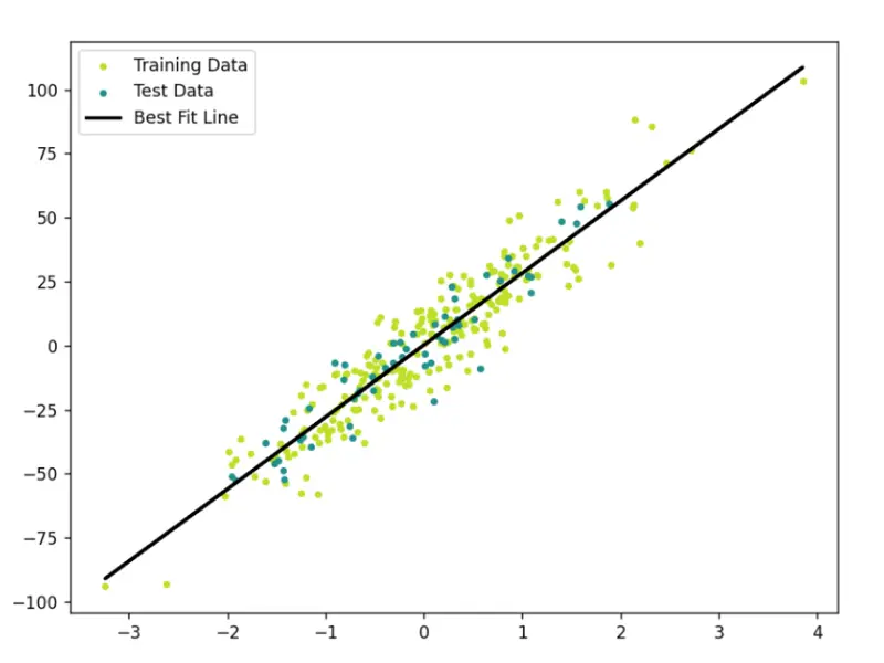
To gain insights, we’ll create a scatter plot with our regression line to visualize the relationship between the variables.

Step 6: Real-world Applications

Linear regression finds applications in predicting housing prices, stock values, and much more. Its simplicity makes it a powerful tool for understanding and predicting real-world phenomena.

Step 7: Coding Linear Regression from Scratch

Now, let’s transition from theory to practice. We’ll code a simple linear regression model in Python, and then evaluate it’s performance on unseen data.
Code can be found on GitHub.

Step 7.1 Importing Libraries:

import numpy as np 
from sklearn import datasets 
from sklearn.model_selection import train_test_split 
import matplotlib.pyplot as plt
  • numpy for matrix operations.
  • datasets from sklearn for generating a regression dataset.
  • train_test_split from sklearn for splitting the dataset into training and testing sets.
  • matplotlib.pyplot for data visualization.

Step 7.2 Define Linear Regression Class:

class Linear_Regression:
    def __init__(self, lr=0.1, n_iters=100):
        self.weights = None
        self.bias = None
        self.lr = lr
        self.n_iters = n_iters

Here we define a class Linear_Regression to encapsulate linear regression functionality. It has an initialization method setting default learning rate (lr) and number of iterations (n_iters). weights is initialized to none because each feature will have its own weight, i.e. no of weights are equal to the no of features. But there will be only 1 bias.

So, if we have n features the equation of our line will be like this:

y = θ0 + θ1X1+ θ2X2 + . . . + θnXn

Step 7.3 Fit Method:

def fit(self, X, y):
    n_samples, n_features = X.shape
    self.weights = np.zeros(n_features)
    self.bias = 0

    for _ in range(self.n_iters):
        '''
            Here,
            fs are features
                 f1  f2   f3  f4  f5  
            X = [x11,x12,x13,x14,x15]  weights = [w1]  bias = bias
                [x21,x22,x23,x24,x25]            [w2]
                [x31,x32,x33,x34,x35]            [w3]
                [x41,x42,x43,x44,x45]            [w4]
                [x51,x52,x53,x54,x55]            [w5]
            '''
        y_pred = np.dot(X, self.weights) + self.bias

        dw = (1/n_samples) * np.dot(X.T, (y_pred - y))
        db = (1/n_samples) * np.sum(y_pred - y)

        self.weights = self.weights - self.lr * dw
        self.bias = self.bias - self.lr * db

The fit method trains the linear regression model using gradient descent. It initializes weights and bias, iteratively updates them to minimize the error.

Step 7.4 Predict Method

def predict(self, X_test):
    predicted = np.dot(X_test, self.weights) + self.bias
    return predicted

Step 7.5 Main Execution Block

def mse(y1, y2):
    return np.mean((y2 - y1)**2)

if __name__ == "__main__":
    # Data Generation and Splitting
    X, y = datasets.make_regression(n_samples=300, n_features=1, noise=10, random_state=42)
    X_train, X_test, y_train, y_test = train_test_split(X, y, test_size=0.2, random_state=3)

    # Model Initialization and Training
    model = Linear_Regression()
    model.fit(X_train, y_train)

    # Model Prediction and Evaluation
    preds = model.predict(X_test)
    print("Mean Squared Error:", mse(preds, y_test))

    # Visualization
    fig = plt.figure(figsize=(8, 6))
    predictions = model.predict(X)
    cmap = plt.get_cmap('viridis')
    plt.scatter(X_train,y_train,color=cmap(0.9),s=10,label='Training Data')
    plt.scatter(X_test,y_test,color=cmap(0.5),s=10,label='Test Data')
    plt.plot(X,predictions,color="black",linewidth=2,label="Best Fit Line")
    plt.legend()
    plt.show()
  • Here we generate a synthetic regression data, splits it into training and testing sets.

  • Initialize the linear regression model.

  • Train the model on the training data.

  • Makes predictions on the test data and evaluates the model using Mean Squared Error.

  • Finally, visualize the training and testing data along with the regression line.

7.6 Best Fit Line:

Best fit line

Points to Note: Common Misconceptions

Misconception 1: Linear Regression Assumes Linearity in All Cases

While linear regression assumes a linear relationship between variables, it doesn’t mean that the variables themselves must be linear. Transformations can be applied to make the relationship linear, even if the original variables are not.

Explanation: This misconception often arises from the name “linear regression.” People may assume that the technique is only applicable when relationships are strictly linear. In reality, it’s about the linearity in the coefficients, not necessarily the raw variables.

Misconception 2: Outliers Always Negatively Affect Linear Regression

While outliers can influence linear regression models, they don’t always have a negative impact. Sometimes outliers contain valuable information or highlight specific patterns in the data.

Explanation: Outliers may disproportionately affect the model if they have a substantial impact on the overall pattern. However, not all outliers are detrimental; they can represent unique scenarios or anomalies that are important to capture.

When to Apply Linear Regression: Key Points to Consider

  1. Linearity: Linear regression is most effective when there is a linear relationship between the input and output variables. Visualizing the data through scatter plots can help identify linearity.

  2. Homoscedasticity: The variance of the errors should be consistent across all levels of the independent variable. If the spread of errors widens or narrows systematically, it indicates heteroscedasticity, which may violate linear regression assumptions.

  3. Independence: Observations should be independent of each other. For example, in time-series data, consecutive observations may be correlated, violating the independence assumption.

  4. Normality of Residuals: The residuals (the differences between actual and predicted values) should be approximately normally distributed. This assumption is important for statistical inference.

Why I Built a Brain for My AI Agents — and What It Taught Me About Memory

`—
title: “Why I Built a Brain for My AI Agents — and What It Taught Me About Memory”
published: true
description: “Anamnesis v0.3.0: The cognitive architecture that emerged when a physician stopped treating agent memory as an engineering problem and started treating it as a clinical one.”
tags: ai, opensource, agents, architecture
cover_image:

canonical_url:

Anamnesis v0.3.0: The cognitive architecture that emerged when I stopped treating agent memory as an engineering problem and started treating it as a clinical one.

Dr. Shweta Patel, MD, FACOG — Board-certified OB/GYN · U.S. Navy veteran (13 yrs) · CEO, Gaya Wellness · 43 AI-leveraged products

TL;DR: Anamnesis is an open-source 4D strategic memory engine for autonomous AI agents. It stores judgment alongside facts — reasoning, authority, trust weight, and decay conditions. Version 0.3.0 adds four brain-inspired capabilities: attention gating, batch consolidation, context-mode retrieval, and prospective memory triggers. The cognitive parallels weren’t planned. Identical problem constraints produced convergent architecture. MIT licensed. Self-hosted. PostgreSQL + pgvector. Deploys in 30 minutes via Docker.

The Problem No One Is Solving

I run an autonomous agent fleet. Forty-three AI-leveraged products across clinical operations, marketing, content production, patient intake, and internal automation. These agents operate around the clock, making thousands of decisions per day.

And every single session started from zero.

Not because the models weren’t smart enough. They were brilliant. The problem was memory-context decoupling — the gap between what an agent knows during a session and what it retains between sessions. It’s the most under-addressed failure mode in autonomous AI, and it produces agents that are perpetually amnesiac. Smart enough to solve any problem. Incapable of remembering they already solved it yesterday.

So I surveyed the landscape. Mem0 stores facts with vector similarity and offers the broadest ecosystem integration — a legitimate production tool. Zep adds temporal knowledge graphs and excels at tracking how entities and relationships change over time. Letta treats memory like an operating system, with the LLM managing its own tiers. All of them solve retrieval: find the relevant thing.

None of them solve judgment: what matters most right now and why.

I needed my agents to remember that enterprise leads convert at 34% — but also why that fact was stored, who determined its importance, how it ranks against competing priorities, and under what conditions it stops being true. Facts without reasoning are trivia. Agents that accumulate trivia don’t get wiser. They get slower.

I Approached This as a Clinician, Not an Engineer

Here’s the thing nobody in the AI memory space seems to be saying: memory-context decoupling is a clinical problem, not an engineering one.

I’ve spent 13 years as a Navy medical officer and over a decade in clinical OB/GYN. When I looked at agent memory loss, I didn’t see a retrieval optimization problem. I saw something I recognized from practice.

Patients with early cognitive decline don’t lose facts first. They lose the weighting of facts. They remember their daughter’s name and their cardiologist’s name, but they can’t tell you which one to call during chest pain. The facts are intact. The judgment layer — what matters, what’s urgent, what to ignore — is what degrades.

That’s exactly what I was watching in my agents. They could retrieve relevant memories. They couldn’t tell me which ones mattered more than others, or why, or when to stop trusting them.

That reframe changed the entire architecture. Instead of building a better filing cabinet, I built Dimension 4: the strategic reasoning envelope. Every memory in Anamnesis carries not just content, but a full reasoning payload: why it was stored, who said so, how important it is relative to everything else, and the explicit conditions under which it expires.

`python

A normal memory system stores the fact:

memory.add(“Enterprise converts at 34% from demo”)

Anamnesis stores the judgment:

client.retain(
bank=”sales_ops”,
content=”Enterprise converts at 34% from demo”,
reasoning=”2x better than SMB. Focus sales energy here.”,
authority=”explicit”, # CEO said this, not inferred
tags=[“revenue”, “enterprise”],
decay_condition=”after:90d”, # revisit in 90 days
)
`

That reasoning field and authority hierarchy are what separate Anamnesis from everything else in this space. When an agent calls reflect(), it doesn’t get a list of similar facts. It gets a ranked operating directive — weighted by strategic importance, with citations and gap analysis. Not a memory dump. A briefing.

The Four Dimensions of Memory

Anamnesis retrieves across four dimensions simultaneously, fused through reciprocal rank fusion with a strategic weight boost:

Dimension Operation What It Finds
Semantic vector similarity Conceptually related memories — “lead prioritization” finds “enterprise converts at 34%”
Temporal time-aware decay Recent and frequently accessed memories, filtered by recency and access patterns
Relational entity graph Connected entities — “API v2 dependencies” finds engineering, enterprise, and pipeline
Strategic weight + reasoning Memories ranked by importance with full reasoning envelopes and authority hierarchy

The first three dimensions — semantic, temporal, relational — exist in various forms across the memory landscape. Dimension 4 is the novel contribution. It’s the layer that turns retrieval into judgment.

The Cognitive Parallels We Didn’t Plan

This is the part that surprised me.

I didn’t set out to model the brain. I set out to make my agents stop being stupid between sessions. But when the architecture stabilized and I started looking at what we’d built, the parallels to human cognitive architecture were everywhere — and they were structural, not superficial.

The thesis: identical problem constraints produce convergent architecture. The brain and Anamnesis solve the same fundamental problem — how to store, weight, retrieve, and prune information under resource constraints so that the most important knowledge surfaces at the right time. When the problem is the same, the solutions converge.

Human Memory Anamnesis Key Insight
Hippocampal encoding retain() Neither system stores raw input. Both extract structured features at encoding time.
Amygdala emotional tagging Strategic envelope Both tag memories with importance metadata that biases all future retrieval.
Multi-cue reconstruction 4D recall + RRF Both retrieve using parallel cues weighted toward importance, not just similarity.
Rehearsal consolidation reweight() Strength is earned through repeated use, not assigned at creation.
Synaptic pruning decay_check Forgetting is a feature. Both systems actively prune to keep retrieval clean.
Prefrontal executive reflect() The layer that transforms remembered facts into actionable judgment.
Source monitoring Authority hierarchy Who said it determines initial trust level.

The convergence isn’t accidental and it isn’t marketing. Research from the intersection of neuroscience and AI has been moving in this direction for years. A 2025 paper in Frontiers in Neural Circuits demonstrated that feedforward projections from sensory cortex to hippocampus function as feature-extracting encoders — the brain doesn’t store raw input, it stores structured representations. That’s exactly what retain() does: fact extraction, entity resolution, embedding generation. We built the same pipeline independently because the problem demands it.

Similarly, a 2025 paper in Neural Networks on the stability-plasticity dilemma proposed AI architectures with dual learning rates and offline consolidation inspired by hippocampal-cortical coordination. They were describing the same pattern we’d already implemented in reweight() and decay_check. Same problem. Same constraints. Convergent solution.

Why this matters: The convergence validates both directions. If the brain’s architecture is a good solution to the memory-under-resource-constraints problem, then AI systems facing the same constraints should converge on similar designs. When they do — independently — it’s evidence the architecture is right.

What’s New in v0.3.0: Four Brain-Inspired Capabilities

Version 0.3.0 completes the cognitive mapping. Each of these four features has a direct parallel to a specific human memory mechanism — and each one solves a specific operational problem I was seeing in production.

🧠 Selective Attention → retain_gate

The brain doesn’t encode everything that hits the retina. Neither should your agent. retain_gate filters inputs before encoding — rejects exact duplicates, warns on semantically similar content, and prevents the context pollution that degrades retrieval quality over time. In production, my agents were storing 3-4 near-identical versions of the same decision. Now they don’t.

💤 Sleep Consolidation → batch_consolidate

During sleep, the hippocampus replays the day’s experiences, merges related memories, detects contradictions, and promotes patterns to long-term storage. batch_consolidate does the same thing on a cron job: merges duplicates, flags contradictions, promotes recurring patterns to higher strategic weight, and produces a consolidation report. Your agent’s overnight maintenance cycle.

🎯 Mood-Congruent Recall → context_mode

Humans in crisis recall different memories than humans in planning mode. Same brain, same memories, different retrieval bias. The context_mode parameter lets you specify an operational state — crisis, planning, review — that biases which memories surface and how they’re weighted. An agent triaging a production outage needs different recall than one doing quarterly planning.

⏰ Prospective Memory → trigger_memory

Prospective memory is the ability to remember to do something in the future: “remind me to check the oven in 20 minutes.” trigger_memory creates semantic tripwires — memories that fire when a future query matches their trigger condition. “When someone asks about API v2, surface the enterprise dependency analysis.” Your agent doesn’t just remember the past. It plants flags for the future.

The Bug That Proved the Architecture

Two weeks before this release, I found a bug that would have been invisible in a simpler system.

The reflect endpoint was producing stale briefings. Not wrong, exactly — but oddly weighted. Old decisions were surfacing above recent ones in contexts where recency should have dominated. I ran a diagnostic using Anamnesis’s own entity heat scoring and temporal analysis. The system told me what was wrong with itself.

The root cause: a temporal score inversion. The scoring function was using last_accessed_at instead of created_at for the temporal dimension, which meant that every time reflect retrieved a stale memory, it refreshed the access timestamp, which made the stale memory score higher in the next retrieval. A feedback loop that reinforced staleness.

Let me be clear about why this matters: the system was self-diagnosable. Because Anamnesis stores reasoning alongside facts, and because the strategic envelope includes temporal metadata, the diagnostic tools could trace exactly why a memory was being overweighted. The entity heat map showed the inversion pattern. The authority hierarchy confirmed no one had explicitly boosted these old memories. The decay conditions had been correctly set but were being bypassed by the access-refresh loop.

This is diagnostic reasoning. It’s the same process I use in clinical practice — the system reveals its own blind spots when you have the right instrumentation. A flat vector store with no reasoning layer would have silently produced degraded results until someone noticed the outputs were off. Anamnesis caught its own disease.

Where This Goes

The immediate use case is obvious: give your AI agents strategic memory. Stop building agents that start every session from zero. Store the reasoning behind decisions so your agents don’t just remember what happened — they remember why it mattered.

But the longer arc is more interesting to me.

The same architecture that gives machines strategic memory can augment human cognition. If you have a patient with early cognitive decline, the facts are still there — it’s the weighting and retrieval prioritization that degrades. What if you connected existing human hardware to an intelligent memory layer that maintained the strategic envelopes? Not replacing memory. Augmenting it. Keeping the judgment intact when the biology starts to slip.

That’s speculative. But it’s why I named this project Anamnesis — the Greek philosophical concept that knowledge is not learned but remembered. The engine gives agents access to judgment they didn’t generate themselves, stored by a planning layer that did. And the same principle might eventually give humans access to judgment their own biology is struggling to maintain.

For now, though: it’s MIT-licensed, self-hosted, deploys in 30 minutes, and it will make your agents meaningfully smarter between sessions.

🔗 Anamnesis v0.3.0 — Open Source

4D Strategic Memory Engine for Autonomous AI Agents
PostgreSQL + pgvector · FastAPI · Docker · MCP Server · Python SDK

⭐ View on GitHub

MIT License · Self-hosted · Deploys in 30 minutes · Star the repo if this is useful

Intelligence knows the answer. Wisdom knows which answer matters. Anamnesis gives your agents wisdom.

Dr. Shweta Patel is a board-certified OB/GYN, 13-year U.S. Navy veteran, author of The Book of Hormones, and CEO of Gaya Wellness, where she leads 43 AI-leveraged products across clinical and operational automation. She built Anamnesis to solve a problem in her own agent fleet and open-sourced it because the memory gap affects everyone building with autonomous agents.`

What Nobody Tells You About Building a Multi-Provider MCP Server

Every MCP server tutorial follows the same script: install the SDK, define a tool, return a response. Ship it.

That works for a single API. It does not work when you need an agent to reliably choose between, authenticate to, and call 645+ different APIs across 86 categories — and handle everything that goes wrong at 3am with no human.

We built Rhumb, an MCP server that proxies hundreds of real APIs for AI agents. Here’s what actually broke, why the tutorials don’t cover it, and what you need to know if you’re building anything beyond hello-world.

Bug #1: The slug aliasing problem

First surprise: APIs don’t have stable identifiers.

Brave’s search API appears as both brave-search-api and brave-search depending on which documentation page you read. When an agent asks to “search with Brave,” your MCP server needs to know these are the same service.

This isn’t unique to Brave. We found alias collisions in payment providers (same company, multiple API versions with different names), communication platforms (SMS vs messaging vs voice — same provider, different “APIs”), and analytics tools (legacy vs v2 naming).

The fix isn’t a lookup table. It’s a canonical slug system with alias resolution that treats identity as a first-class problem.

Why tutorials skip this: They show one API. You never hit naming collisions with one API.

Bug #2: Authentication is not a solved problem

The tutorials say: “Add your API key to the header.” That covers maybe 40% of real APIs.

What we actually encountered across providers:

  • Bearer token (Authorization: Bearer {key}) — ~45% of services
  • Custom header (X-API-Key, X-Subscription-Token, Api-Key) — ~25%
  • Basic Auth (base64 encoded credentials) — ~15%
  • OAuth2 with token refresh — ~10%
  • Query parameter (?api_key=…) — ~5%

The problem isn’t supporting all five patterns. It’s that your MCP server needs to know which pattern each API uses before the agent’s first call. If the agent sends a Bearer token to an API expecting X-API-Key, you get a 401 that tells the agent nothing useful.

Worse: some APIs accept the wrong auth method silently and return empty results instead of errors.

Bug #3: The payload translation trap

Your agent constructs a JSON payload. The API expects multipart form data.

This hits hardest with document processing APIs. An agent wants to send a file for parsing. It constructs a reasonable JSON body with the file content. The API returns 400 because it only accepts multipart uploads with specific field names.

The gap between “what the agent naturally produces” and “what the API actually accepts” is wider than anyone admits:

  • Parameter naming: query vs q vs search_query vs prompt
  • Body format: JSON vs form-encoded vs multipart
  • Array handling: tags=a,b,c vs tags[]=a&tags[]=b vs {"tags": ["a","b"]}
  • Date formats: ISO 8601 vs Unix timestamps vs custom strings
  • Pagination: cursor vs offset vs page-number vs link-header

Why this matters for agents: A human developer reads the docs and adapts. An agent will retry the same malformed request until it hits rate limits.

Bug #4: Error messages that lie

Here’s a real error response from a production API:

{"error": "An error occurred. Please try again later."}

An agent receiving this will try again later. The actual problem? Invalid API key format. Retrying will never help.

The quality gap in error responses across 645+ APIs is staggering:

Good (Stripe-class):

{
  "error": {
    "type": "invalid_request_error",
    "code": "parameter_missing",
    "param": "amount",
    "message": "Missing required param: amount"
  }
}

Bad (more common than you’d think):

{"status": "error", "message": "Bad Request"}

In our scoring of 645+ APIs, structured error responses are a minority. Most APIs return human-readable error strings that agents can’t reliably parse.

Bug #5: Rate limits without information

Good APIs tell you exactly where you stand:

X-RateLimit-Limit: 1000
X-RateLimit-Remaining: 247
X-RateLimit-Reset: 1616000000
Retry-After: 30

Bad APIs return 429 and nothing else.

Some APIs have undocumented secondary rate limits. GitHub’s REST API has a primary rate limit (5,000/hour) and a secondary rate limit on “content-creating” endpoints that’s lower and not reflected in headers. An agent creating issues or comments will hit the secondary limit and get a 403 with a message about “secondary rate limits” that doesn’t appear in any getting-started guide.

Real numbers from our data:

  • Stripe (AN 8.1): Rate limit headers, Retry-After, burst limit documented
  • GitHub (AN 7.8): Primary headers yes, secondary limits documented but not in headers
  • PayPal (AN 4.9): Headers inconsistent, sandbox limits undocumented

Bug #6: The sandbox illusion

“Just use the sandbox.” Every API says this. Few deliver.

Real sandbox problems we encountered:

  • Sandbox requires production credentials — defeats the purpose
  • Sandbox has different behavior — you test against a lie
  • Sandbox has stricter rate limits — can’t performance test
  • Sandbox doesn’t support all endpoints — partial testing only
  • Sandbox requires CAPTCHA to create — agents can’t self-provision

PayPal’s sandbox requires CAPTCHA verification to create accounts. That one detail drops it from “agent-friendly” to “requires a human for setup.”

Bug #7: The versioning time bomb

APIs change. Versioning is supposed to protect you.

In practice:

  • Stripe: Explicit API version in every request header. Pin a version, get consistent responses forever.
  • Most APIs: Unversioned endpoints that change without notice. Your agent’s response parser breaks silently when email_address becomes emailAddress.

The insidious part: breaking changes often affect edge cases first. Your happy-path tests pass. Your agent hits the edge case at 3am.

What we learned

After building through all of this, we distilled the problems into a scoring framework. Every API gets evaluated on 20 dimensions:

Execution (70%): Error handling, schema stability, idempotency, latency, rate limit transparency.

Access Readiness (30%): Signup friction, auth complexity, docs quality, sandbox, rate limits.

Some results that surprised us:

  • Stripe (8.1) and Twilio (8.0) are genuinely built for automation
  • GitHub (7.8) is excellent but has sneaky secondary rate limits
  • Resend (7.8) — newer email API that got the details right from day one
  • SendGrid (6.4) — dominant but showing age in error handling
  • PayPal (4.9) — the CAPTCHA sandbox alone is disqualifying for autonomous use
  • Salesforce (4.8) — powerful but the OAuth dance is hostile to agents

The full leaderboard across 86 categories is at rhumb.dev/leaderboard.

If you’re building an MCP server

  1. Treat service identity as a first-class problem. You will hit naming collisions.
  2. Build an auth resolution layer. Don’t make the agent know which header format each API uses.
  3. Expect payload translation. What the agent sends and what the API wants are rarely the same shape.
  4. Parse errors defensively. Most APIs don’t return structured errors.
  5. Implement rate limit tracking per-provider. Don’t share a single backoff strategy.
  6. Test against production, not just sandboxes. Many sandboxes are incomplete.
  7. Pin API versions where possible. If the API doesn’t support versioning, monitor for breaking changes.

The MCP protocol gives you a great transport layer. It tells you nothing about what happens when your tools hit real APIs. That part is on you.

Rhumb scores 645+ APIs across 86 categories on 20 dimensions. Methodology at rhumb.dev/methodology. MCP server is open source: github.com/supertrained/rhumb.

We scanned 4,162 MCP servers. 73% are invisible to AI agents.

There are 4,162 MCP servers registered on Smithery right now. The Python and TypeScript SDKs see 97 million monthly downloads. Every major AI provider has adopted MCP.

But nobody had measured the quality of these tools.

We built ToolRank, an open-source scoring engine that analyzes MCP tool definitions across four dimensions. Then we pointed it at the entire Smithery registry.

The biggest finding wasn’t about quality. It was about visibility.

73% of MCP servers are invisible

Out of 4,162 registered servers, only 1,122 expose tool definitions that agents can read.

The remaining 3,040 — 73% — have no tool definitions at all. They’re registered, but when an AI agent searches for tools, these servers don’t exist. They have no name, no description, no schema. They are invisible.

This is the equivalent of having a website with no indexable content. Google can’t rank what it can’t read. Agents can’t select what they can’t see.

Among the visible: average score 84.7/100

For the 1,122 servers that do expose tool definitions, we scored each one across four dimensions:

Dimension Weight What it measures
Findability (25%) Can agents discover you? Registry presence, naming
Clarity (35%) Can agents understand you? Description quality, purpose, context
Precision (25%) Is your schema precise? Types, enums, required fields
Efficiency (15%) Are you token-efficient? Definition size, tool count

Average ToolRank Score: 84.7/100

Level Score Count %
Dominant 85-100 677 60%
Preferred 70-84 406 36%
Selectable 50-69 39 3.5%
Visible 25-49 0 0%
Absent 0-24 0 0%

The average is higher than expected. But there’s a survivorship bias: servers that bother to expose tool definitions tend to be better maintained overall. The real quality problem is the 73% that expose nothing.

Top scoring servers

Rank Server Score
1 microsoft/learn_mcp 96.5
2 docfork/docfork 96.5
3 brave (Brave Search) 94.7
4 LinkupPlatform/linkup-mcp-server 93.5
5 smithery-ai/national-weather-service 93.3

What do top servers do differently? They start descriptions with clear action verbs. They include usage context (“Use this when…”). They define required fields, enums, and defaults. They keep tool count under 15.

The most common defects

Among the 1,122 scored servers, the most frequent issues:

  1. Missing usage context — Description says what the tool does, but not when to use it. Agents need “Use this when…” to decide between competing tools.

  2. No return value described — Agents can’t predict what they’ll get back. This leads to incorrect downstream handling.

  3. Missing parameter descriptions — Schema has types but no explanations. An agent sees "query": {"type": "string"} but doesn’t know what format the query should be in.

  4. No required fields defined — Agents guess which parameters are mandatory, leading to failed executions.

  5. Description too short — Under 50 characters. Not enough information for reliable selection.

What does this mean?

Academic research backs up why this matters. A study of 10,831 MCP servers (arXiv 2602.18914) found that tools with quality-compliant descriptions achieve 72% selection probability vs 20% for non-compliant ones. That’s a 3.6x advantage.

The fixes are trivial. Adding “Use this when…” to a description. Defining required fields. Starting the description with a verb. These are 5-minute changes with measurable impact.

We’re calling this ATO

ATO (Agent Tool Optimization) is the practice of optimizing tools so AI agents autonomously discover, select, and execute them.

SEO optimized for search engines. LLMO optimized for LLM citations. ATO optimizes for agent tool selection.

The key difference: SEO and LLMO result in mentions and links. ATO results in your API being called and transactions occurring. LLMO is Stage 1 of ATO — necessary but not sufficient.

Full ATO framework →

Try it yourself

Score your tools: toolrank.dev/score — paste your tool definition JSON. Includes “Try example” buttons so you can see how scoring works instantly.

Ecosystem ranking: toolrank.dev/ranking — live rankings updated weekly.

Scoring engine: github.com/imhiroki/toolrank — fully open source. The scoring logic is transparent.

Methodology

  • Data source: Smithery Registry API (registry.smithery.ai)
  • Scan date: March 28, 2026
  • Servers in registry: 4,162
  • Servers with tool definitions: 1,122 (27%)
  • Scoring level: Level A (rule-based, 14 checks, zero LLM cost)
  • Request interval: 2 seconds (respectful to Smithery infrastructure)
  • Full scan time: ~2 hours
  • Code: Open source

Data updates weekly via automated scanning. Daily differential scans catch new servers.

Built by @imhiroki. Questions, feedback, or want to improve your score? Open an issue on GitHub.

DAG vs Langraph Nodes

When we have DAG that represents our tasks and its dependencies do we still need Langraph nodes?

LangGraph nodes are most valuable when your flow has cycles — loops, retries, HITL resume, conditional branching back to earlier steps. A pure DAG has none of that, so LangGraph’s core value proposition doesn’t apply.

So are they mutually exclusive? No! They can complement each other. See the beautiful project to understand why.

LangGraph nodes for the orchestration layer: intent_parser → entity_extractor → plan_builder → hitl_plan → cot_builder → hitl_confirm. This is the stateful, cyclic part.

Your own DAG executor for task execution: takes the confirmed TaskGraph, runs a topological sort, fans out independent tasks with asyncio, collects results. Twenty to thirty lines of plain Python. No framework.

fixing two bugs stacked on top of each other in ProseMirror

heading joins with par

i’m building a markdown editor built on Milkdown (which wraps ProseMirror). i hit a bug in how marks behave when you join blocks together.

the bug

type a bold heading. move your cursor to the start of it. press Backspace. the heading joins into the paragraph above, but the bold marks bleed into the previously-unstyled paragraph text.

heading joins with par

i assumed this was a bug in joinTextblockBackward. it wasn’t.

what’s actually going on

when you press Backspace at position 0 of a textblock, joinTextblockBackward fires. under the hood, joinTextblocksAround calls:

replaceStep(state.doc, beforePos, afterPos, Slice.empty)

this deletes the boundary between the two blocks. the Fitter algorithm stitches the content of the second block into the first. it doesn’t touch inline marks. the text nodes transfer as-is, bold and all.

there’s a clearIncompatible function that strips marks disallowed by the target node type, but paragraphs allow bold, so nothing gets stripped. there’s also splitBlockKeepMarks which handles the reverse operation (Enter), but that’s about storedMarks — cursor behavior for the next typed character. different problem.

so the marks survive the join, and they’re supposed to. consider two paragraphs:

She said the results were
**statistically significant** and could not be ignored.

press Backspace at the start of the second paragraph. they merge into one. the bold must survive because you put it there intentionally. if ProseMirror stripped marks on join, it would destroy user content.

the heading case feels wrong for a different reason. in a markdown editor, # **Bold Heading** has explicit bold marks on the text nodes because that’s what the markdown source says. you see the boldness as part of the heading, like a visual property of the block. but ProseMirror sees it as an inline mark that happens to sit inside a heading node. the markdown editor stores the heading’s visual weight in two places: the node type and the inline marks. when the heading unwraps into a paragraph, only the node type changes. the marks stay because ProseMirror doesn’t know they were “heading-ness” and not “the user explicitly wanted bold.”

not a ProseMirror bug. a modeling problem specific to markdown editors.

the fix

i intercept joinTextblockBackward‘s dispatch. before the transaction reaches the editor state, i snapshot the heading content range, then append removeMark calls for the region that used to be the heading. i also clear storedMarks so the cursor doesn’t inherit marks either. everything lands in one transaction, so undo reverses it atomically.
heading joins correctly with no mark bleed

here’s the standalone plugin:

import { Plugin, PluginKey } from "prosemirror-state";
import { joinTextblockBackward } from "prosemirror-commands";

const headingBackspacePlugin = new Plugin({
  key: new PluginKey("heading-backspace"),
  props: {
    handleKeyDown(view, event) {
      if (event.key !== "Backspace") return false;

      const { state, dispatch } = view;
      const headingType = state.schema.nodes.heading;
      if (!headingType) return false;

      const { $from, empty } = state.selection;
      if (
        !empty ||
        $from.parentOffset !== 0 ||
        $from.node().type !== headingType
      )
        return false;

      // Snapshot before the join mutates anything.
      const headingContentSize = $from.node().content.size;
      const prevEnd = $from.before();

      const wrappedDispatch = (tr: typeof state.tr) => {
        // Map prevEnd through the join's ReplaceStep to find where
        // the heading content now sits inside the merged paragraph.
        const from = tr.mapping.map(prevEnd);
        const to = from + headingContentSize;

        // Strip every mark type from the former-heading range.
        for (const markType of Object.values(state.schema.marks)) {
          tr.removeMark(from, to, markType);
        }

        // Clear storedMarks so the cursor doesn't inherit marks.
        tr.setStoredMarks([]);

        dispatch(tr);
      };

      return joinTextblockBackward(state, wrappedDispatch, view);
    },
  },
});

$from.before() gives the position just before the heading’s opening token — after the join’s ReplaceStep deletes the block boundary, tr.mapping.map(prevEnd) gives the new position where the heading content starts inside the merged paragraph. headingContentSize is stable because the join doesn’t change the heading’s content, just moves it. tr.removeMark is safe to call multiple times on the same transaction and tr.setStoredMarks([]) clears cursor marks so typing after the join doesn’t inherit bold/italic. the whole thing is one transaction — Ctrl+Z undoes the join and the mark removal together.

if you’re using Milkdown or Tiptap, register this through the framework’s plugin API. the ProseMirror logic is identical.

related discussion