Linux Performance Tuning: CPU, Memory, I/O & Network

Linux performance optimization covers four major subsystems:

Subsystem Typical Bottleneck Scenario
CPU Compute-intensive workloads (Nginx, Node.js, math/batch processing)
Memory Database workloads (MySQL) — heavy memory and storage consumption
I/O Disk-bound applications with heavy read/write
Network High-throughput web services

Section 1: CPU Performance

CPU is the most critical subsystem — responsible for all computation. Modern production servers use multi-core CPUs based on SMP (Symmetric Multiprocessing) architecture. In practice, CPU utilization is often below 5%, meaning significant resource waste.

CPU Cache Hierarchy

# lscpu
L1d cache:   32K    ← L1 data cache (static, per-core)
L1i cache:   32K    ← L1 instruction cache (static, per-core)
L2 cache:    256K   ← dynamic, shared
L3 cache:    8192K  ← dynamic, shared across cores
  • L1 cache: static cache, split into data and instruction caches
  • L2 / L3 cache: dynamic cache; L2 is shared between cores

CPU Affinity

In SMP systems, the Linux scheduler may run the same thread on different cores across time slices. Since each core has its own memory space (not shared), this causes cache invalidation — the thread’s data must be reloaded into the new core’s cache, degrading performance.

CPU affinity pins a process to a specific core, maximizing cache hit rate:

# Pin process 73890 to CPU core 0
taskset -pc 0 73890

NUMA (Non-Uniform Memory Access)

taskset alone doesn’t guarantee local memory allocation. For NUMA architectures, use numactl:

NUMA topology:
┌──────────────┐     ┌──────────────┐
│  CPU Node 0  │     │  CPU Node 1  │
│  Local RAM   │     │  Local RAM   │
│  (fast)      │     │  (fast)      │
└──────┬───────┘     └──────┬───────┘
       │  remote access (slower)  │
       └──────────────────────────┘
# View current NUMA configuration
numactl --show

# Bind program to specific NUMA node
numactl --cpunodebind=0 --membind=0 ./myapp

⚠️ Database servers should NOT use NUMA by default. If required, start the DB with numactl --interleave=all to avoid memory hotspots.

CPU Scheduling Policies

Real-time scheduling (priority 1–99, higher = more urgent):

Policy Behavior
SCHED_FIFO Static priority; once running, holds CPU until higher-priority task arrives or it yields
SCHED_RR Round-robin with time slices; expired slice goes to end of queue — fair among equal-priority tasks

General scheduling (priority 100–139, lower number = higher priority):

Policy Behavior
SCHED_OTHER Default; priority determined by nice + counter values. Least recently scheduled gets priority.
SCHED_BATCH For batch processing
SCHED_IDLE For very low priority background tasks
# Adjust process priority with nice (-20 to 19, lower = higher priority)
renice 5 <pid>

# Modify real-time scheduling priority
chrt -r -p 50 <pid>

Context Switches

The Linux kernel treats each core as an independent processor. Each core can run 50–50,000 processes. Each thread gets a time slice; when it expires or is preempted, a context switch occurs.

The more context switches, the heavier the kernel scheduling overhead.

Run Queue

Each CPU has a run queue. A thread is either sleeping (blocked on I/O) or runnable (waiting for CPU time).

load = currently running threads + threads in run queue

Example: 2 cores, 2 running + 4 queued → load = 6

CPU Performance Targets

Healthy CPU metrics:
┌─────────────────────────────────────────┐
│  us (user)    60% – 70%                 │
│  sy (system)  30% – 35%                 │
│  id (idle)     0% –  5%                 │
│  run queue    ≤ 4 per core (ideal)      │
└─────────────────────────────────────────┘
# Monitor with vmstat (1-second intervals, 5 samples)
vmstat 1 5
procs -----------memory---------- ---swap-- -----io---- --system-- -----cpu------
 r  b   swpd   free   buff  cache   si   so    bi    bo   in   cs  us  sy  id  wa
 3  0 1150840 271628 260684 5530984  0    0     2     1    0    0  22   4  73   0
 5  0 1150840 270264 260684 5531032  0    0     0     0  5873 6085 13  13  73   0

High in (interrupts) and cs (context switches) indicate the kernel is constantly switching processes and servicing hardware requests.

Bind Interrupts to a Specific CPU

# Bind interrupt type 19 to CPU core 2
echo 03 > /proc/irq/19/smp_affinity

# Bind TCP interrupts to one CPU (reduces scheduler interference)

Section 2: Memory Performance

Linux uses Virtual Memory Management (VMM) — writes go to filesystem cache in memory first, then flush to disk lazily. This is why available memory appears low after running Linux for a while: most is consumed by cache + buffer.

Optimization goal: reduce disk writes, improve write efficiency.

Dirty Data Flush Policy

# Trigger pdflush when dirty data exceeds 10% of physical memory
echo 10 > /proc/sys/vm/dirty_background_ratio

# Flush dirty data that has been in memory longer than 2000ms
echo 2000 > /proc/sys/vm/dirty_expire_centisecs

⚠️ Tune carefully — these settings have a large impact on I/O performance.

Swap Tuning

When physical memory is insufficient, Linux uses LRU to swap out cold pages to disk, and swap in when needed.

# 0 = prefer physical memory; 100 = aggressively use swap
echo 10 > /proc/sys/vm/swappiness   # recommended for production

Minimize swap usage in production. For Redis, disable overcommit:

echo 0 > /proc/sys/vm/overcommit_memory

Reclaiming Memory

sync
echo 3 > /proc/sys/vm/drop_caches
# 1 = drop page cache (buffers)
# 2 = drop slab cache (cached)
# 3 = drop both

Huge Pages

Large page sizes reduce TLB misses and page table overhead:

cat /proc/meminfo | grep -i huge
# AnonHugePages: transparent huge pages (auto-managed)
# Hugepagesize:  2048 kB (standard huge page size)

# Manually set huge page count
sysctl vm.nr_hugepages=20

32-bit: 4MB huge pages; 64-bit: 2MB huge pages.
Larger pages = less overhead but more internal fragmentation.

Page Faults

MPF (Major Page Fault):  data not in cache → read from disk (expensive)
MnPF (Minor Page Fault): data found in buffer cache → no disk I/O (cheap)
# First run: mostly MPF (cold cache)
/usr/bin/time -v ./myapp

# Second run: mostly MnPF (warm cache)
/usr/bin/time -v ./myapp

The File Buffer Cache continuously grows to reduce MPF and increase MnPF, until the kernel needs to reclaim memory for other processes. Low free memory ≠ memory pressure — Linux intentionally uses free memory for caching.

Section 3: Disk I/O Performance

The I/O subsystem is typically the slowest part of a Linux system — both due to physical distance from the CPU and mechanical/electrical constraints. Minimize disk I/O wherever possible.

I/O Scheduler

cat /sys/block/sda/queue/scheduler
# noop  anticipatory  deadline  [cfq]
Scheduler Description Best For
CFQ (default) Completely Fair Queuing; up to 8 requests per time slice; idles waiting for more I/O from same process General workloads
Deadline Every request must be served before a deadline Databases, latency-sensitive
noop No scheduling; FIFO order SSDs, VMs
anticipatory Deprecated; good for write-heavy/read-light Legacy

I/O Priority

# Set process I/O priority (1=realtime, 2=best-effort, 3=idle)
ionice -c1 -p <pid>   # highest I/O priority for pid

Page Size & Block Size

Linux kernel accesses disk I/O in pages (typically 4KB):

/usr/bin/time -v date   # shows page size info

Tune page size and block size based on your application’s I/O pattern (large sequential vs. small random).

DMA (Direct Memory Access)

DMA allows hardware to transfer data directly to/from memory without CPU involvement:

Without DMA: disk → CPU → memory  (CPU occupied during transfer)
With DMA:    disk ──────▶ memory  (CPU free during transfer)

DMA transfer lifecycle: Request → Acknowledge → Transfer → Complete

Writing Data Back to Disk

# Force immediate flush
fsync()   # per-file
sync()    # system-wide

# pdflush runs periodically if not explicitly called

Useful I/O Monitoring Commands

iotop      # per-process I/O usage
lsof       # list all open files and file descriptors
iostat     # disk I/O statistics
vmstat     # combined system stats including I/O

Section 4: Network Performance

For web applications, network performance is critical. Potential bottlenecks include: application response time, Linux network subsystem, NIC, and bandwidth.

NIC Settings

# Check if NIC is in full-duplex mode
ethtool eth0

# Increase MTU for high-bandwidth (≥1Gbps) networks
ifconfig eth0 mtu 9000 up   # jumbo frames

TCP Buffer Tuning

# TCP read buffer: min / initial / max (bytes)
sysctl -w net.ipv4.tcp_rmem="4096 87380 8388608"

# TCP write buffer: min / initial / max (bytes)
sysctl -w net.ipv4.tcp_wmem="4096 87380 8388608"

TCP Window Scaling

# Disable window scaling and set fixed window size
# (similar to setting JVM -Xms = -Xmx for predictability)
sysctl -w net.ipv4.tcp_window_scaling=0

TCP Connection Reuse

Reusing TIME_WAIT connections avoids the full 3-way handshake overhead — significant performance gain for web servers:

sysctl -w net.ipv4.tcp_tw_reuse=1
sysctl -w net.ipv4.tcp_tw_recycle=1

Keepalive Timeout

# Release idle persistent connections sooner (default is much longer)
sysctl -w net.ipv4.tcp_keepalive_time=1800   # 1800 seconds

SYN Backlog (DoS Protection)

# Max length of queue for TCP connections not yet ESTABLISHED
# Prevents server crash under SYN flood / DoS attacks
sysctl -w net.ipv4.tcp_max_syn_backlog=4096

Disable Unnecessary Protocols

# Disable ICMP broadcast responses to reduce noise
sysctl -w net.ipv4.icmp_echo_ignore_broadcasts=1

Bind Network Interrupts to One CPU

# Bind NIC interrupt to CPU core 1 (reduces scheduler interference)
echo 02 > /proc/irq/<nic_irq>/smp_affinity

Recommended Monitoring Toolset

Tool Purpose
htop Interactive process and CPU monitor
vmstat CPU, memory, swap, I/O, context switches
iotop Per-process disk I/O
sar Historical system activity reports
strace Trace system calls for a process
iftop Real-time network bandwidth by connection
ss Socket statistics (faster replacement for netstat)
lsof List open files and file descriptors
ethtool NIC diagnostics and settings
mtr Combined traceroute + ping for network diagnosis

Why the AI sprint planning market is solving the wrong problem

In the last six months, at least four tools have launched promising to plan your dev sprint with AI. I’ve looked at all of them closely — not as a competitor, but because I want to understand what problem this market thinks it’s solving.

Here’s the pattern: every single one optimizes for planning quality. Better backlog prioritization, smarter task sequencing, AI-generated sprint goals, roadmap visualization. They’re genuinely well-built products.

And they will not help you ship.

The planning problem isn’t the planning

METR published a study in July 2025 that measured what actually happened when experienced software developers used AI tools on real engineering tasks. The result surprised a lot of people: they were 19% slower than without AI assistance.

The explanation isn’t that AI tools are bad. It’s that experienced devs spent time evaluating AI suggestions, second-guessing their own instincts, adjusting output. The overhead of managing the AI ate the time savings.

The same dynamic plays out in sprint planning tools. You open the app. You spend 25 minutes getting a really good sprint plan. The plan is genuinely better than what you would have built yourself.

Then you close the tab.

Not because the plan was wrong. Because a plan is inert. It doesn’t produce the state change you need to actually open your editor at 9pm after a full-time job and work on your side project.

What the tools don’t have

I mapped the four main tools against what I think the actual problem is:

AgileTask tells you what to build this week. It does not know you haven’t opened your editor since Tuesday.

MVP Copilot gives you a sprint structure. It does not have a fixed end date with a consequence if you miss it.

LaunchChair gives you a launch roadmap. It does not have milestone checkpoints where a human reviews what you actually shipped.

MVPable generates your MVP plan in 60 seconds. It does not follow up when you disappear.

The gap isn’t planning quality. The gap is the Witness Effect.

What the Witness Effect actually is

This isn’t a new concept. Accountability research has documented it consistently: when someone else knows you’re supposed to do a thing, your follow-through rate is measurably higher than when you’re accountable only to yourself. Not because of peer pressure in the negative sense — because human social cognition is wired to treat external observation as real in a way that internal commitment isn’t.

Private to-do lists don’t produce this. Streak counters don’t produce this. Community feeds where you post when you feel like it don’t produce this.

What produces it: a specific person who reads your daily check-in, knows what you were supposed to have built by Day 13, and notices when you stop showing up.

One data point

Cohort #1, Silver tier. Ghulam, GPS flight planner for DJI drones. Before the sprint: stuck on an architectural decision for two months.

Day 13 milestone: Leaflet map with KML export live on GitHub Pages. 532 waypoints. Litchi import working for DJI Air 2S.

He didn’t get unstuck because the daily prompts were clever. He got unstuck because he had a deadline and someone on the other side of it.

The tools that plan your sprint well have gotten very good. The category that checks whether you followed through is mostly empty.

That’s what I’m building. If you want to look at it: mvpbuilder.io

How to Apply to 100 Jobs in One Afternoon (Without Sending Junk)

The advice you’ll find everywhere is: quality over quantity. Tailor every resume. Research every company. Craft every cover letter.

That advice was written for a different market.

In 2025, recruiting benchmarks from Gem’s dataset of 140 million applications showed that candidates are roughly three times less likely to be hired today than they were three years ago. Pass-through rates are dropping. Interviews per hire are rising. Time to hire is getting longer.

The math has changed. Quality still matters. But volume now matters too.

The problem: if tailoring one resume takes 20 minutes, applying to 100 jobs takes 33 hours. That’s a full work week just on applications. Most people can’t do that. So they either blast an untailored resume everywhere, or they apply to 10 jobs carefully and wait.

Neither works very well.

There’s a third option.

The Batch Approach

The core idea: do your tailoring work in batches instead of one application at a time.

Instead of: pick job, tailor resume, apply, pick next job, repeat.

You do: collect 20-30 job URLs, process all of them at once, submit in sequence.

This sounds small, but it changes everything about how you spend your time and energy.

Step 1: Build Your Job List First (30-45 minutes)

Most people open a job board, see a role, and immediately start applying. This is inefficient. You context-switch constantly and never build momentum.

Instead, spend 30-45 minutes doing nothing but collecting jobs.

Open LinkedIn, Indeed, or whatever boards you use. Search for your target roles. Open each listing that looks relevant. Copy the URL. Paste it into a spreadsheet.

Your criteria at this stage should be loose: does this role roughly match what you do? If yes, save it. You’re not committing to applying yet. You’re building a list.

Aim for 30-50 jobs per session. This sounds like a lot. It isn’t. At 1-2 minutes per listing, that’s 30-60 minutes of searching.

Once your list is done, go through and eliminate obvious mismatches. You’ll probably cut 20-30%. What’s left is your batch.

Step 2: Prepare One Strong Base Resume (one-time, 1-2 hours)

If you haven’t done this yet, do it now. A base resume is your starting point: your full experience, your best bullet points, your accomplishments in their strongest form.

This is the document you tailor from, not the document you submit.

A few things that make tailoring faster later:

  • Write each bullet point in outcome language (“increased X by Y,” not “responsible for X”)
  • Include more detail than you’ll submit (you’ll cut to fit, not add)
  • Keep it in a format that’s easy to edit (Google Docs or Word, not PDF)

You only do this once. Every application after this is a variation of this document.

Step 3: Process the Batch (the actual bulk apply)

Now you work through your job list. For each role:

  1. Open the job description
  2. Identify the 3-5 most repeated keywords or phrases
  3. Check your base resume: do your bullet points reflect this language?
  4. Rephrase any bullets that can be improved without being dishonest
  5. Rewrite your 2-3 line summary to match this specific role
  6. Export and submit

If you’re doing this manually, each application takes 15-20 minutes once you have the method down. A batch of 20 jobs takes 4-6 hours. Spread over two days, that’s manageable.

If you’re using a tool that automates steps 2-5, a batch of 20 jobs can take under an hour. I built BulkResumes for exactly this: paste your base resume, paste a list of job URLs, and it generates individually tailored resumes and cover letters for each one. The underlying logic is the same as the manual method, just automated.

Either way, the batch approach is the same. You’re not rushing. You’re removing the setup overhead that makes individual applications feel so slow.

What “Tailored” Actually Means at Scale

There’s a fear that applying to 100 jobs means sending 100 generic resumes. It doesn’t have to.

Tailoring has a spectrum:

  • Generic (same resume, zero changes): works only if you’re extremely well-matched to every role
  • Light tailoring (summary rewritten, 2-3 bullet points rephrased): takes 10 minutes, meaningfully increases relevance
  • Deep tailoring (every section customized, company research incorporated): takes 60-90 minutes, appropriate for high-priority roles

The batch approach doesn’t mean you always do light tailoring. It means you sort your applications by priority and allocate effort accordingly.

Tier 1 (your top 5-10 roles): deep tailoring. Research the company. Write a specific cover letter. Spend the time.

Tier 2 (solid matches): standard tailoring. 15-20 minutes each.

Tier 3 (stretch or speculative): light tailoring. Summary plus 2 bullets. Submit and move on.

Most people only have a Tier 1 mindset. They apply to 10 jobs as if they were all dream jobs, then give up when nothing happens. The batch approach forces you to think in tiers and get things moving.

The Quality Check That Actually Matters

There’s one thing that kills bulk applications: submitting resumes with errors, wrong company names, or copy-paste artifacts from previous tailoring.

Before each submission:

  • Read the first paragraph of your summary out loud. Does it sound like it was written for this job?
  • Check that your resume doesn’t still say the previous company name or role anywhere
  • Confirm contact info and formatting are intact

That’s it. Two minutes. Anything more and you’re over-optimizing.

The Honest Reality

Volume without targeting is noise. If you’re applying to every job on the board regardless of fit, you’ll get a response rate of near zero and burn out fast.

Volume with basic targeting and light tailoring is signal. You’re showing up in relevant searches, your resume language matches what they’re looking for, and you’re submitting enough applications that the math works in your favor.

The goal isn’t 100 applications. The goal is 100 relevant applications with resumes that aren’t working against you.

In a market where you’re three times less likely to be hired than a few years ago, that means you need to apply to more jobs than before, tailor more consistently than before, and waste less time per application than before.

The batch approach gives you all three.

A Simple System to Start Today

  1. Today (30 min): Build a list of 20-30 jobs you’re genuinely qualified for. Don’t apply yet.
  2. Tomorrow morning (2 hrs): Polish your base resume so it’s strong on its own.
  3. Tomorrow afternoon (2-3 hrs): Work through your batch. Tailor and submit each one.
  4. Repeat weekly: New batch every Monday. Track what you sent. Follow up on anything that goes quiet after 2 weeks.

That’s roughly 10-15 applications a week done properly, or 40-60 a month. In a tough market, that’s enough volume to get the math working for you.

Start with the list.

How ATS Actually Filters Your Resume (And What to Do About It)

Here’s a number that should make you uncomfortable: 88%.

That’s the share of employers who told Harvard Business School and Accenture, in a landmark 2021 study called “Hidden Workers”, that their applicant tracking system had rejected qualified, high-skilled candidates purely because they didn’t tick the right filter boxes. For middle-skilled roles? 94%.

So the meme about “ATS killing your resume” isn’t paranoia. It’s documented. The question is: what are you going to do about it?

Let’s actually look inside the machine.

What ATS Is (and Isn’t)

ATS, applicant tracking system, is software that companies use to collect, organize, and rank job applications. The big names are Workday, Greenhouse, Lever, iCIMS, Taleo. If you’ve ever filled in a “careers portal” form and manually re-typed everything that was already on your resume… that’s ATS eating your data.

Here’s the thing most guides get wrong: ATS isn’t one universal algorithm that scores your resume 0-100 and rejects the losers. It’s closer to a searchable database with filters layered on top. A recruiter posts a job, sets up filters (minimum years of experience, must-have keywords, education requirements), and the system hides applications that don’t pass.

The filtering can be aggressive or basically nonexistent, it depends entirely on how the company configured it. But the failure modes are consistent enough that we can talk about them.

The Two Ways Your Resume Gets Killed Before a Human Sees It

Failure Mode 1: Parsing failure

Before your resume gets ranked or filtered, ATS has to read it. This is called parsing, the system extracts your text and turns it into structured data: name, contact info, job titles, dates, skills.

If your resume uses tables, text boxes, multi-column layouts, graphics, or contact info in the header/footer section, the parser may extract garbage. Your five years of engineering experience might not register. Your name might land in the “skills” field. You’ll never know, because the portal says “application received” regardless.

Resume parsing software has gotten better, but “better than it was in 2015” still doesn’t mean it handles creative formatting gracefully. Clean, boring formatting wins.

Failure Mode 2: Keyword matching failure

Once parsed, your resume gets matched against what the recruiter is looking for. This is mostly keyword matching, does your resume contain the specific words and phrases in the job description?

Most ATS systems are not doing deep semantic analysis. They’re checking whether “project management” appears in your resume when the job description says “project management.” If your resume says “led cross-functional initiatives,” that might not register, even though it means the same thing.

This is why job seekers with genuinely relevant experience still get filtered out. They’re writing their experience in their vocabulary, not the employer’s.

The Fix: Two Minutes Before You Submit Anything

Step 1, Format check (60 seconds):

  • Single-column layout only. No tables, no text boxes, no graphics.
  • Contact info in the body of the document, not in a Word header/footer (parsers often skip those).
  • Standard section headings: “Work Experience,” “Education,” “Skills.” Not “My Story” or “What I’ve Built.”
  • File format: DOCX is safer for portals. PDF is fine when you’re emailing directly to a person.

Step 2, Keyword check (60 seconds per application):
Read the job description. Find the 5-8 most repeated or bolded terms. Check if those exact terms (or close variations) appear in your resume.

If you have the underlying experience but used different words, rephrase. “Managed client relationships” becomes “client relationship management” if that’s what the job description says. You’re not lying. You’re translating.

That’s it. You don’t need to “optimize for ATS” beyond this. Most ATS guides on the internet are selling complexity on what is, at its core, a formatting and vocabulary problem.

What ATS Can’t Touch, And Why That Part Is Harder

ATS gets you into the visible pile. After that, a human recruiter looks at what’s in front of them.

The average recruiter skim lasts about 6-7 seconds. They’re checking: does this person’s title/background make sense for this role? Is there a recognizable company name or credential? Does the career trajectory make sense?

Here’s the uncomfortable truth: keyword-optimized resumes that get past ATS but have weak substance still don’t get interviews. ATS optimization is the floor, not the ceiling.

The ceiling is a resume where your actual work, quantified, specific, clearly stated, is compelling to a human who reads it in under 30 seconds.

The Scaling Problem

Here’s where it gets annoying.

Every job has different keywords. If you’re doing this properly, you’re rephrasing 3-5 bullets and rewriting your summary for each application. Manual. Every. Time.

For 5 jobs a week, that’s totally doable, maybe 30-40 minutes of work spread across a few days.

For 20-30 jobs a week (which is what it takes to reliably get responses in a tough market), you’re looking at several hours just on resume variants. Most people don’t do it. They submit the same resume everywhere and get frustrated when the response rate sits at 2-3%, which, for the record, is completely normal.

If you’re applying at volume, BulkResumes handles the keyword matching and rephrasing step automatically. Upload your base resume, paste in your target job descriptions, and get individually tailored resumes back, each one using the vocabulary of that specific role. The ATS logic is baked in.

Whether you do it manually or with a tool: match their words, keep your format clean, and don’t let a parser silently discard work you actually did.

The Short Version

  • ATS is a database with filters, not a single algorithm
  • Parsing failure kills resumes before humans see them, fix with clean, single-column formatting
  • Keyword failure filters out relevant candidates, fix by mirroring the job description’s language
  • 88% of employers have filtered out qualified people this way (Harvard/Accenture, 2021)
  • The fix is two minutes of formatting checks + keyword matching per application
  • At volume, this becomes a time problem, which is what automation is for

Designing a Production-Oriented RAG System for Technical Documentation

Large Language Models are incredibly powerful, but they have a major limitation:

They do not inherently know your infrastructure, your internal documentation, your deployment standards, or your engineering workflows.

Generic LLMs can explain concepts like Docker, Terraform, or NGINX at a broad level, but when building real engineering systems, broad knowledge is not enough. Engineering teams need:

  • accurate retrieval,
  • contextual understanding,
  • domain-specific responses,
  • conversational continuity,
  • and reliable citations.

That is where Retrieval-Augmented Generation (RAG) systems become important.

This article explores the architecture and implementation of the RAG pipeline built for VizLab.xyz — an internal AI-powered documentation assistant and developer copilot designed around real engineering workflows.

Instead of functioning as a generic chatbot, the system was designed to:

  • retrieve highly relevant technical documentation,
  • maintain conversational context,
  • reduce hallucinations,
  • provide citation-backed answers,
  • and operate entirely within a controlled documentation ecosystem.

The architecture combines:

  • FastAPI
  • FAISS
  • BM25
  • AWS Bedrock
  • AWS Titan Embeddings
  • Docker
  • Tailscale
  • Caddy Reverse Proxy
  • S3-backed vector persistence

while remaining lightweight enough to self-host on a private infrastructure stack.

Why Traditional LLMs Fail for Engineering Workflows

One of the biggest problems with using general-purpose LLMs in technical environments is hallucination.

A model may:

  • generate outdated commands,
  • invent configuration syntax,
  • confuse versions,
  • or answer from unrelated training data.

For engineering environments, this is dangerous.

If a system generates:

  • incorrect Terraform configurations,
  • invalid NGINX directives,
  • broken IAM policies,
  • or misleading Docker instructions,

the consequences can directly affect infrastructure stability.

The goal of the VizLab RAG system was therefore not to create a “smart chatbot.”

The goal was to create a retrieval-first architecture where:

  1. trusted documentation is indexed,
  2. relevant context is retrieved,
  3. and the LLM is forced to answer primarily from that retrieved context.

This architectural approach significantly improves response reliability.

System Goals

The system was specifically designed for:

  • internal technical documentation retrieval,
  • educational AI workflows,
  • developer assistance,
  • DevOps troubleshooting,
  • infrastructure guidance,
  • and conversational technical support.

The indexed knowledge base includes curated documentation from domains such as:

  • Docker
  • NGINX
  • Terraform
  • GitHub Actions
  • Solidity
  • AWS Policies
  • Infrastructure tooling

Rather than scraping the entire internet, the system intentionally targets a highly curated set of engineering documentation sources.

This dramatically improves:

  • retrieval precision,
  • chunk quality,
  • and contextual relevance.

High-Level Architecture

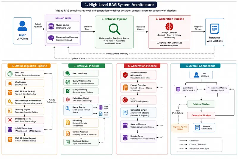
The architecture is divided into three major pipelines:

  1. Offline Ingestion Pipeline
  2. Retrieval Pipeline
  3. Generation Pipeline

The complete architecture diagram is shown below.

Step 1: Documentation Scraping

The system begins by scraping a curated list of documentation URLs using BeautifulSoup.

Instead of indexing random internet pages, the scraper focuses on trusted engineering sources.

Examples include:

  • Docker documentation
  • Terraform documentation
  • NGINX references
  • AWS documentation
  • Solidity references

This dramatically improves knowledge quality.

One important architectural decision was storing raw scraped content immediately into AWS S3 before processing.

This provides:

  • durability,
  • backup recovery,
  • ingestion reproducibility,
  • and debugging visibility.

If chunking or embedding pipelines fail, raw documentation is still preserved.

Step 2: Text Cleaning & Normalization

Raw documentation contains:

  • navigation elements,
  • repeated menus,
  • headers,
  • footers,
  • formatting artifacts,
  • inconsistent whitespace.

Before chunking, the pipeline normalizes and cleans the content.

This stage improves:

  • embedding quality,
  • retrieval relevance,
  • and token efficiency.

Garbage input produces garbage embeddings.

Cleaning matters more than many people realize.

Step 3: Chunking Strategy

One of the most important parts of any RAG system is chunking.

The VizLab pipeline uses a recursive text splitting strategy designed to preserve semantic meaning.

Poor chunking destroys retrieval quality.

If chunks are:

  • too small → context becomes fragmented
  • too large → embeddings become noisy
  • overlapping incorrectly → retrieval becomes redundant

The system therefore uses overlapping semantic chunks to preserve continuity across boundaries.

This allows the retrieval system to maintain:

  • contextual coherence,
  • command relationships,
  • and infrastructure explanations.

The indexed system currently maintains roughly:

  • 300–500 chunks,
  • 300–500 embeddings,
  • with a FAISS index smaller than 5MB.

Because the dataset is intentionally curated and focused, retrieval quality remains high without massive storage overhead.

Step 4: Embedding Generation

After chunking, the documents are converted into vector embeddings using AWS Titan Embeddings through Amazon Bedrock.

Embeddings convert semantic meaning into numerical vector representations.

This enables similarity search based on meaning rather than exact keyword matching.

For example:

A user asking:

“How do I configure reverse proxying?”

can still retrieve chunks mentioning:

  • upstream routing,
  • proxy_pass,
  • load balancing,
  • or NGINX forwarding,

even if the exact wording differs.

Why Hybrid Search Was Used

One of the most important architectural decisions was combining:

  • FAISS dense retrieval
  • with BM25 sparse retrieval.

Dense vector search is excellent for:

  • semantic understanding,
  • paraphrased questions,
  • conceptual similarity.

But dense retrieval sometimes struggles with:

  • exact command syntax,
  • specific keywords,
  • infrastructure flags,
  • version identifiers.

BM25 solves this by ranking exact keyword relevance.

Combining both systems creates a hybrid retrieval architecture that balances:

  • semantic similarity,
  • and exact-match retrieval.

Here is the Reciprocal Rank Fusion (RRF) logic that combines both lists:

@staticmethod
def _rrf_merge(
    dense: list[RetrievedChunk],
    sparse: list[RetrievedChunk],
    k: int = 60,
) -> list[RetrievedChunk]:
    """
    Reciprocal Rank Fusion.
    RRF score = Σ 1 / (k + rank_i)
    """
    rrf: dict[str, RetrievedChunk] = {}

    for rank, chunk in enumerate(dense, start=1):
        if chunk.chunk_id not in rrf:
            rrf[chunk.chunk_id] = chunk
        rrf[chunk.chunk_id].rrf_score += 1.0 / (k + rank)
        rrf[chunk.chunk_id].faiss_score = max(
            rrf[chunk.chunk_id].faiss_score, chunk.faiss_score
        )

    for rank, chunk in enumerate(sparse, start=1):
        if chunk.chunk_id not in rrf:
            rrf[chunk.chunk_id] = chunk
        rrf[chunk.chunk_id].rrf_score += 1.0 / (k + rank)
        rrf[chunk.chunk_id].bm25_score = max(
            rrf[chunk.chunk_id].bm25_score, chunk.bm25_score
        )

    return sorted(rrf.values(), key=lambda c: c.rrf_score, reverse=True)

This significantly improves engineering query performance.

Especially for:

  • CLI commands,
  • configuration syntax,
  • infrastructure tooling,
  • and troubleshooting workflows.

Retrieval Pipeline

Once ingestion is complete, the system becomes queryable.

The retrieval pipeline is responsible for:

  • understanding user intent,
  • retrieving relevant context,
  • and assembling prompt-ready information.

Query Cache Layer

Before entering retrieval, queries first pass through an LRU TTL cache.

If an identical query already exists, the system bypasses:

  • vector retrieval,
  • embedding generation,
  • and LLM invocation.

Cached responses return in under 5ms.

This dramatically reduces:

  • Bedrock API usage,
  • latency,
  • and infrastructure cost.

Caching becomes especially important in developer environments where:

  • repeated troubleshooting questions,
  • repeated configuration lookups,
  • and repeated deployment issues

occur frequently.

Conversational Memory System

The conversational memory implementation uses an in-memory sliding-window architecture.

Each session maintains:

  • recent user messages,
  • assistant replies,
  • timestamps,
  • and conversational ordering.

The memory system stores:

  • 6 user turns
  • and 6 assistant turns

before automatically truncating older context.

This sliding-window approach prevents:

  • prompt explosion,
  • token overflows,
  • and degraded retrieval quality.

The memory subsystem influences two separate stages:

1. Query Rewriting

If a user asks:

“How do I configure that for NGINX?”

the retriever analyzes previous messages to understand what “that” refers to.

This significantly improves retrieval accuracy for follow-up conversations.

2. Prompt Compilation

The conversation history is also injected into the final LLM prompt.

This enables conversational continuity while keeping context size controlled.

The implementation currently uses:

  • an in-memory Python dictionary,
  • mapped by session_id.

This architecture is lightweight and extremely fast for single-instance deployments.

However, for multi-replica scaling, this would eventually need migration to:

  • Redis,
  • or another distributed memory layer.

Query Rewriting

One major issue with naive RAG systems is weak query formulation.

Users rarely ask perfectly structured questions.

The VizLab system expands queries into multiple search variants before retrieval.

This dramatically improves recall.

For example:

A query like:

“How do I secure my containers?”

may internally generate variants related to:

  • Docker security
  • container isolation
  • runtime permissions
  • capabilities
  • reverse proxy security
  • TLS hardening

The implementation for expanding queries looks like this:

def _rewrite_query(self, query: str, intent: str, domains: list[str]) -> list[str]:
    """Expand the query into search-optimised variants."""
    rewrites = [query]
    q_lower = query.lower()

    if intent == "debug":
        rewrites.append(f"{' '.join(domains)} {q_lower} causes fix solution")
        rewrites.append(f"troubleshoot {q_lower}")
    elif intent == "how_to":
        rewrites.append(f"{q_lower} step by step guide configuration")
        rewrites.append(f"{'  '.join(domains)} {q_lower} example")

    # Cross-domain context injection
    if len(domains) > 1:
        rewrites.append(f"{' '.join(domains)} integration {query}")

    return list(dict.fromkeys(rewrites))

This improves retrieval coverage substantially.

Re-Ranking Pipeline

After retrieval, results are re-ranked based on:

  • keyword density,
  • contextual relevance,
  • freshness,
  • and semantic confidence.

Without re-ranking, vector systems often retrieve:

  • partially related chunks,
  • noisy semantic neighbors,
  • or overly broad context.

To solve this, a custom re-ranking step applies domain-specific heuristic boosts:

def _rerank(self, chunks: list[RetrievedChunk], qu: QueryUnderstanding) -> list[RetrievedChunk]:
    """
    Boost chunks by:
      +0.1 per exact keyword match in chunk text
      +0.05 if chunk domain matches query domain
      +0.05 if chunk is Section 0 (intro / overview)
    """
    q_keywords_lower = {k.lower() for k in qu.keywords}
    for chunk in chunks:
        text_lower = chunk.text.lower()

        # Keyword density bonus
        keyword_hits = sum(1 for kw in q_keywords_lower if kw in text_lower)
        chunk.rrf_score += keyword_hits * 0.1

        # Domain match bonus
        if chunk.metadata.get("domain") in qu.domains:
            chunk.rrf_score += 0.05

        # Introductory chunk bonus
        if chunk.metadata.get("chunk_index", 99) == 0:
            chunk.rrf_score += 0.05

    return sorted(chunks, key=lambda c: c.rrf_score, reverse=True)

Re-ranking significantly improves response precision.

Prompt Engineering & Hallucination Control

One of the hardest engineering problems during development was strict citation enforcement.

Amazon Bedrock Titan occasionally attempted to answer from:

  • its base model training,
  • rather than the retrieved documentation context.

This is a common RAG failure mode.

The solution required:

  • strict system prompts,
  • structured prompt assembly,
  • guardrails,
  • context enforcement,
  • and fallback validation logic.

The final prompt compiler injects:

  • retrieved context,
  • system instructions,
  • conversation history,
  • user query,
  • and formatting constraints

into a single structured payload.

The model is heavily instructed to answer primarily from retrieved context.

This significantly reduces hallucinations and improves citation reliability.

Why Streaming Responses Were Avoided

Many AI systems use token streaming.

This architecture intentionally avoids it.

Instead, the system waits for the complete generation before returning a strict JSON payload.

Why?

Because the system prioritizes:

  • citation integrity,
  • structured outputs,
  • deterministic formatting,
  • and response validation.

Streaming complicated reliable citation attachment.

For technical documentation systems, correctness was prioritized over token-by-token rendering speed.

Deployment Architecture

The entire RAG service is containerized using Docker.

The backend stack includes:

  • FastAPI
  • Gunicorn
  • AWS Bedrock
  • FAISS
  • Caddy
  • Tailscale

The infrastructure is fully self-hosted.

Importantly:
the backend is never directly exposed to the public internet.

Instead:

  • the service operates inside a private Tailscale network,
  • secured behind a Caddy reverse proxy.

Caddy was specifically chosen because it integrates cleanly with Tailscale and automatically manages TLS certificates inside the private mesh network.

This removed significant operational overhead.

Request Lifecycle Walkthrough

A typical request flows through the following stages:

  1. User submits query from frontend UI
  2. Request enters Tailscale-secured network
  3. Caddy proxies request to FastAPI backend
  4. Query cache checks for existing response
  5. Conversational memory enriches context
  6. Query rewriting expands retrieval scope
  7. FAISS + BM25 perform hybrid search
  8. Retrieved chunks are re-ranked
  9. Prompt compiler assembles final payload
  10. AWS Bedrock Titan generates response
  11. Structured JSON response returned to frontend
  12. Response stored in memory and cache

This entire process currently averages around:

~8.9 seconds end-to-end latency.

What Broke During Development

The hardest parts of the project were not the LLM APIs.

The hardest parts were infrastructure and operational consistency.

1. Dockerizing FAISS & Bedrock Dependencies

Packaging the ingestion pipeline inside Docker caused repeated failures during CI/CD.

The challenge was getting:

  • Python dependencies,
  • FAISS native bindings,
  • Bedrock credentials,
  • and ingestion runtime behavior

to work consistently inside the container environment.

This took extensive debugging across:

  • container startup,
  • dependency compatibility,
  • and runtime initialization.

2. Tailscale + Caddy Networking

One of the most painful debugging sessions involved:

  • reverse proxying,
  • CORS,
  • Tailscale networking,
  • and frontend-backend communication.

Ensuring:

  • correct TLS handling,
  • proper headers,
  • secure private networking,
  • and browser compatibility

required multiple iterations.

Networking problems are often far harder than application logic.

3. Prompt Instability

Early versions of the system occasionally ignored retrieved context and answered generically.

This produced:

  • weak citations,
  • hallucinated explanations,
  • inconsistent formatting.

The solution required extensive prompt engineering and retrieval refinement.

This reinforced an important lesson:

In RAG systems, retrieval quality matters more than model size.

Future Improvements

Several improvements are planned for future iterations:

  • distributed vector databases
  • semantic caching
  • Redis-backed distributed memory
  • streaming retrieval pipelines
  • reranking models
  • agentic retrieval workflows
  • observability dashboards
  • tracing and telemetry
  • Kubernetes-native deployment
  • multi-user access control
  • prompt injection detection

The current architecture intentionally prioritizes:

  • correctness,
  • reliability,
  • retrieval quality,
  • and operational simplicity

over premature scaling complexity.

Final Thoughts

Building RAG systems is not simply:

“connecting an LLM to a vector database.”

Production-oriented retrieval systems require:

  • retrieval engineering,
  • chunking strategy,
  • ranking pipelines,
  • conversational memory,
  • prompt control,
  • infrastructure reliability,
  • and operational debugging.

The most valuable lesson from building this architecture was understanding that AI systems are fundamentally systems engineering problems.

Not just machine learning problems.

The quality of:

  • retrieval,
  • infrastructure,
  • networking,
  • caching,
  • and prompt orchestration

ultimately determines whether the system feels reliable in real-world engineering workflows.

And as RAG architectures continue evolving, the engineering surrounding retrieval pipelines may become even more important than the models themselves.

Building in public, week 9: cross-links, positions going up, and 246 new dev.to followers in 7 days

tl;dr: Week 9 was infrastructure week. Closed the biggest SEO gap internal cross-links on 100% of pages. Average position improved for the first time in a month.

The numbers

Metric Week 8 Week 9
Indexed URLs 72 75
Impressions (3 months) 463 509
Avg. position 43.8 40.1
Cross-links coverage 40/64 64/64
dev.to followers 156 402

GA last 7 days: 36 active users (+56.5%), 61 sessions (+38.6%). Traffic sources: Google organic is now the consistent #1.

What I actually did

Cross-links: 40 -> 64/64 ✅

This was the main P0 for the week. Convertify has 64 landing pages (62 format-pair conversions + home + images-to-pdf). In week 8, only 40 had contextual cross-links inline <a href> inside the body text pointing to related conversions.

I added 2-3 cross-links per page across the remaining 24 pages, batched over Monday–Wednesday. The links are semantic, not just alphabetical a page about AVIF->JPG links to AVIF->PNG and JPG->AVIF, not to BMP->TIFF.

The effect on positions isn’t instant. Internal links take 1-2 crawl cycles to register. But average position went from 43.8 to 40.1 the first improvement in a month. Expecting more in T10–T11 as Googlebot re-crawls.

Semrush on-page fixes

Four pages got H1/title/meta updates based on Semrush priority scores:

  • avif-to-webp priority 3.35 (highest), added missing semantic terms
  • avif-to-png priority 0.78, H1 and title now contain “avif to png” exactly
  • heif-to-jpg priority 0.48, body + H1 + title now include “heif image converter”
  • avif-to-jpg priority 0.19, title updated to match “online convert avif to jpg”

Also simplified readability on 4 pages (Semrush flagged them as “difficult to read”) shorter sentences, fewer compound clauses.

Content gaps closed

4 pages brought from 5 to 6+ sections, 2 pages got FAQ expanded from 6 to 8 questions. Home page schema_faq synced (was 4 questions in JSON-LD, 7 in the DB now 7 everywhere).

Also added a comparison table to /images-to-pdf the only page that was missing one.

Google confirmed 35 canonical fixes

Got an email from Google Search Console team confirming that the canonical issues I fixed in T8 (35 pages were flagged as “Alternate page with proper canonical tag”) have been resolved. The “Variant page with canonical tag” count dropped to 0.

SaaSworthy listing

Added Convertify to SaaSworthy full listing (Basic Details + Media + Pricing + FAQs). Free tier was actually free, no “Talk to Us” required.

Pinterest

Created an account, verified the domain via meta tag, published 3 pins:

  • HEIC->JPG: “Convert HEIC to JPG Free Online No Signup”
  • AVIF->PNG: “Convert AVIF to PNG Free Preserve Transparency”
  • PNG->WebP: “Convert PNG to WebP Free 30% Smaller Files”

Not expecting traffic from this. Image search visibility is the goal AVIF and WebP pages might surface in Pinterest search for people looking for format examples.

What I deliberately didn’t do

Researched whether adding “Last updated: May 2026” to pages would help CTR. Found two case studies showing it hurt CTR by 13-22% on tool pages. Probably because it signals the tool is old and was manually touched, not that it’s actively maintained. Skipped it.

The unexpected thing: dev.to followers +246 in one week

I publish weekly “Building in public” posts on dev.to + a technical article each week. Week 9 posts:

  1. “Building in public, week 8: impressions exploded 71% and I think I know why”
  2. “AVIF encoding speed”.

The AVIF article is the one that seems to have triggered the follower spike. It’s pure technical content benchmarks comparing AVIF encoding speed at different quality settings across formats. No promotion, no “check out my tool.” Just data.

My theory: dev.to surfaces content in the weekly digest or the tag feeds, and technical posts about specific formats get picked up by people in the web performance / image optimization community. The followers are probably devs who bookmarked the article and followed for future posts.

What’s not working

Clicks aren’t moving. The pages are showing up in Google avif-to-png has 85 impressions, avif-to-jpg has 66, png-to-webp has 59. But average position is still ~40. Need to be in top 20 for these before clicks appear. The on-page and cross-link work is aimed at exactly this.

Plan for week 10

Keyword targeting on top pages: avif-to-png, avif-to-jpg, png-to-webp are the three pages with the most impressions. These need to move from position ~40 to position ~20. That means: content depth, more FAQ, better semantic coverage, maybe longer-form sections.

The honest take

  • Cross-links: was at 62.5% coverage, now 100%
  • Content: 0 pages below minimum threshold
  • Schema: all mismatches resolved

The position improvement (43.8 -> 40.1) is the first concrete signal that the on-page work is landing. 509 impressions.
Real clicks need top-20 positions. That’s the only thing that matters in T10.

Convertify is a free image converter built with Rust + libvips and Next.js SSG. convertifyapp.net

Week 1–9 archive: dev.to/serhiizahornyi

How I keep LLMs on a tight leash and stopped hand-creating 30 GitHub issues in the process

The way I keep LLMs on a tight leash is through structured issue breakdowns. In this post you’ll see how I go from concept to issue breakdown to GitHub issues to code – and why that sequence makes it easier to run an orchestrator agent directing a focused executor agent without it hallucinating scope.

It starts with a planning doc: a problem statement and a list of items dissecting the solution. Below you’ll see how to turn that into GitHub issues with labels, milestones, and acceptance criteria – without copy-pasting each one by hand.

You copy-paste the first five, by issue eight you are making typos… by issue fifteen you have a duplicate and by issue twenty you have stopped caring about the body format entirely.

I was refactoring a multi-model NLP sentiment classifier from a flat src/ folder into a proper package structure – eight packages, 30+ issues, 3 phases. Every time the plan changed I was back to copy-pasting so I decided to write a 300-line Python CLI to end that.

The result: gh-issue-creator. Give it a JSON template or a plain markdown planning file, it discovers your repo automatically, runs dry by default and even skips issues that already exist. One command, done.

The problem

Most developers plan in text. GitHub Issues wants structured input via a web form or API calls: the gap between those two surfaces is where time disappears.

The GitHub CLI (gh) already handles authentication and API calls cleanly. The missing layer is a thin converter that takes a batch of planned issues — from wherever they live — and creates them with one command.

The constraints I set:

  1. Dry-run by default. Never touch the API without explicit intent.
  2. Read markdown natively. My planning docs are already in ### Issue #50 - Title format. The tool should parse that directly.
  3. Skip duplicates by title. Running the script twice should not create duplicates.
  4. Zero config on a correctly authenticated machine. gh repo view already knows the repo.
  5. Fail loudly and early. Validation errors before any API call, not halfway through a 30-issue batch.

This structure matters even more when the executor is an AI agent. A well-scoped issue with a clear Acceptance section is a bounded task. A vague one is an invitation for the agent to hallucinate scope. The tool forces you to write tight issues before you run anything.

How it works

Two input formats, one output

The tool accepts JSON or markdown. The JSON format gives you full control: labels, assignees, milestones per issue. The markdown format is a convenience parser for when your plan already exists as a doc.

The markdown parser reads headings like ### Issue #50 - Your title and treats everything below each heading as the issue body:

pattern = re.compile(
    r"^###s+Issues+#(?P<number>d+)s*-s*(?P<title>.+?)s*$"
    r"(?P<section>[sS]*?)(?=^###s+Issues+#d+s*-|^##s+|Z)",
    flags=re.MULTILINE,
)

The lookahead ((?=^###s+Issues+#d+s*-|^##s+|Z)) stops at the next issue heading rather than a fixed delimiter — because planning docs don’t have consistent separators.

If you pass a .json path that doesn’t exist but a sibling .md file does, the tool uses it silently. The template path is the default argument and markdown is the natural planning format.

Deduplication before creation

_existing_titles fetches up to 1,000 issues from the target repo before creating anything:

def _existing_titles(repo: str) -> dict[str, int]:
    data = _run_gh([
        "issue", "list", "--repo", repo,
        "--state", "all", "--limit", "1000",
        "--json", "title,number",
    ])
    issues = json.loads(data)
    return {issue["title"]: issue["number"] for issue in issues}

One API call up front, O(1) dict lookup per issue. If the title already exists, it logs the existing issue number and skips. No duplicates even if you run the script twice.

Dry-run is the default

--create must be explicitly passed. Without it, the script logs every planned issue with its metadata and exits without touching GitHub:

if not args.create:
    details = []
    if labels:
        details.append(f"labels={labels}")
    if assignees:
        details.append(f"assignees={assignees}")
    if milestone:
        details.append(f"milestone={milestone}")
    suffix = f" [{', '.join(details)}]" if details else ""
    planned.append(f"- {title}{suffix}")
    continue

The first time I ran a batch tool without a dry-run step and created five duplicate issues on a test repo, I added it immediately.

Lessons learned

  1. Dry-run by default is not extra engineering. It is the minimum viable trust for any tool that writes to a shared API.
  2. Markdown is a planning format. JSON is an API format. Tools that force you to convert your planning format into an API format before they will accept input are adding friction, not removing it. Meet engineers where they already are.
  3. subprocess.run(check=True, capture_output=True) is the right pattern for CLI composition. Let the subprocess fail loudly. Catch CalledProcessError at the call site and print a clean error. Don’t swallow it.
  4. Delegate to existing tools. _discover_repo() is three lines because it just calls gh repo view. Reimplementing remote detection would have been twenty lines and two edge cases I hadn’t thought of.
  5. Tight issues are better context than long prompts. When you hand an executor agent a well-formed GitHub issue — Goal, Scope, Acceptance — it has less room to drift than when you paste a paragraph of instructions. The discipline of writing issues before coding pays double when the coder is an LLM.

No install required

The script uses only Python stdlib — argparse, json, re, subprocess, pathlib. No pip install, no virtualenv.

curl -O https://raw.githubusercontent.com/lfariabr/gh-issue-creator/main/issue_creator.py
curl -O https://raw.githubusercontent.com/lfariabr/gh-issue-creator/main/examples/template.example.md

# dry-run
python issue_creator.py --template template.example.md --repo owner/your-repo

# create
python issue_creator.py --template template.example.md --repo owner/your-repo --create

The repo is at github.com/lfariabr/gh-issue-creator. The README includes three AI agent prompts for delegating the entire workflow — from writing the plan to creating the issues — to a coding agent. That’s the loop: plan in markdown, issues on GitHub, agent on a tight leash.

Clone it, run a dry-run, open a PR if you extend it to handle sub-tasks or GitHub Projects boards.

Why Runtime Reality Breaks Static Assumptions

Most AI systems today reason about infrastructure as if it is static.

A snapshot of:

  • code
  • configs
  • schemas
  • deployment definitions

But real systems are not static.

They evolve constantly.

Sometimes intentionally.

Sometimes because somebody made a “temporary workaround” 11 months ago and now the company is emotionally dependent on it.

The Gap Between “Declared” and “Running”

There is always a gap between:

What is declared

  • Terraform
  • CloudFormation
  • CDK
  • configs
  • architecture diagrams nobody updated since 2023

What is actually running

  • hotfixes
  • partial rollouts
  • deprecated services still somehow alive
  • environment drift
  • shadow dependencies
  • “temporary” scripts promoted directly into production

AI systems mostly reason over the declared layer.

Production lives in the running layer.

That mismatch is where infrastructure assumptions start becoming dangerous.

Drift Is Normal, Not Exceptional

One thing I’ve learned from real systems:

Drift is not some rare edge case.

Drift is the default operating mode of infrastructure.

Schemas drift.
Queues get reused.
Lambda responsibilities quietly expand.
Environment configs diverge.
Feature flags outlive entire product strategies.

And somehow the system still works through a combination of:

  • operational experience
  • institutional memory
  • monitoring alerts
  • and collective engineering anxiety

The problem is:
AI systems usually do not have access to any of that context.

Why This Breaks AI Reasoning

If an AI agent assumes:

  • an index exists because Terraform references it
  • a queue is active because code imports it
  • a service is healthy because it appears in configs
  • an API contract is current because docs mention it

…it can confidently generate completely wrong operational decisions.

Not because the syntax is bad.

Because the system model is stale.

And stale infrastructure assumptions are dangerous precisely because they often look reasonable.

Static Context Has a Ceiling

This is why I think purely static approaches eventually hit a ceiling for infrastructure-heavy AI systems.

You can absolutely improve things with:

  • better retrieval
  • larger context windows
  • repo indexing
  • schema awareness
  • dependency graphs

All of that helps.

But eventually runtime reality wins.

Because production systems are living systems.

Not snapshots.

Runtime Truth Is Hard

To reason reliably about infrastructure, AI systems eventually need awareness of:

  • runtime state
  • deployment reconciliation
  • drift detection
  • evolving dependencies
  • environment divergence
  • operational anomalies

In other words:

what is actually true right now.

Not:

what was declared six months ago and hopefully still exists.

That is a much harder problem than code generation.

But it is also the problem that matters most once software reaches production scale.

This Is the Direction I Keep Thinking About

A lot of the thinking behind Infrawise started from this gap between:

  • static infrastructure definitions
    and
  • operational system reality

Right now I’m mostly exploring deterministic infrastructure context through:

  • schema relationships
  • infra mapping
  • dependency awareness
  • static analysis
  • topology understanding

But long-term I think runtime observability and operational signals become important too.

Because infrastructure awareness is not just:

“what does the code say?”

It is:

“what is the system actually doing?”

Closing

Current AI coding assistants are already very good at understanding source code.

The next generation will need to understand:

  • runtime behavior
  • operational state
  • infrastructure drift
  • deployment reality
  • evolving system relationships

Because production systems are not static architecture diagrams.

They are constantly moving targets held together by software, infrastructure, and a surprising amount of engineering optimism.

How Engineers and Consultants Lose 15 Minutes Every Morning (And What to Do About It)

You open your laptop. You need the inspection report from last week. You know it exists. You saved it yourself.

But where?

Was it in the OneDrive project folder? The network drive? The local Projects directory? Did you email it to yourself at some point? Is there a copy on the desktop from when you needed to edit it quickly?
You spend three minutes finding it. Then you need the Excel load calculation that goes with it. Another two minutes. Then the CAD drawing the client sent. Another two.

Most engineers know the feeling intimately: six File Explorer windows open simultaneously, each navigated to a different folder, none of them closed because closing means losing the location. It is not disorganisation. It is a coping mechanism for a system that offers no better way to hold multiple places at once.

You haven’t done a single minute of actual work yet. You’ve just been navigating folders. This is not a you problem. This is a structure problem.

See how Deckspace solves this in 2 minutes:

How Files Actually Get Scattered
The way most professionals store files makes complete sense in isolation. CAD files go on the network drive because that’s where the licence server is. Client correspondence lives in OneDrive because it needs to be shared. Working files stay local because the network is slow. Downloads pile up in the Downloads folder because that’s the default.

Each decision is logical. The result is chaos.

A single project say, a structural inspection for a bridge might have files in six different locations simultaneously, one in working folder, another in the “reference folder” “client docs” etc. There is no single place to go. There is only the mental overhead of remembering where each piece lives.

For engineers and consultants juggling three or four active projects at once, this compounds fast. The cognitive load of maintaining a mental map of where everything is stored is real, invisible, and exhausting.

Why Folder Structures Don’t Solve It
The standard advice is to build a clean folder structure. One top-level folder per project. Subfolders by document type. Consistent naming conventions.

This works until it meets reality.
Reality is a client who sends files via email. A colleague who drops something on the shared drive in the subfolder that is most relevant for the organisation. A CAD file that has to live on the network drive regardless of your folder hierarchy. A downloaded PDF you forgot to move.

Folder structures are fragile because they depend on every file ending up in the right place every time. They break the moment the real world gets involved, which is immediately and always.
The deeper problem is that Windows organises files by location. You work by project. Those two things are fundamentally misaligned, and no folder structure fixes that mismatch, it just manages it.

The Actual Cost
Fifteen minutes a day finding files is a conservative estimate for anyone running multiple simultaneous projects.

Across a five-day work-week that is over an hour. Across a year it is more than sixty hours. A full working week and a half spent doing nothing except navigating a file system that was not designed for the way you work.

That number does not include the subtler cost: the context switching. Every time you go hunting for a file, you lose the thread of what you were doing. Getting back into deep focus after an interruption takes time. The file hunt is not just fifteen minutes. It is fifteen minutes plus the recovery time.

What Actually Helps
The fix is not a better folder structure. It is decoupling project organisation from file location.

Instead of moving files into the right place, you keep files wherever they naturally live and create a project-based view on top. The files stay on the network drive, in OneDrive, on the desktop, wherever they are. You simply maintain a workspace that connects them together under a project context.

This is how tools like Deckspace approach the problem. Rather than asking you to reorganise your file system, it lets you create project workspaces where you drag in links to your actual files, portals, in the app’s language. The file stays where it is. The portal remembers the connection. Open your Bridge Upgrade workspace and every file for that project is right there, regardless of which drive it actually lives on.

The original files are untouched. The folder structure your IT department mandates is untouched. Nothing moves. You just stop having to remember where everything is.

A Practical Starting Point
Whether you use a dedicated tool or not, the principle holds: stop trying to force your files into a single location and start building a project-based index on top of wherever they live.

If you are on Windows, the simplest version of this is a pinned folder in Quick Access for each active project, with shortcuts to the most-used files inside. It is manual and fragile but it is better than nothing.

The more robust version is a tool that maintains those connections persistently, survives file moves with a relink, keeps notes and comments attached to individual files, and shows you exactly what you opened and when.

Either way, the goal is the same: open your laptop in the morning and go directly to your project. Not to a folder tree. Not to a search bar. To the work itself.

Fifteen minutes a day is too much to spend looking for things you already have.

Deckspace is a file workspace manager for Windows and macOS. It lets you create project workspaces and drag files from anywhere on disk into them as portal shortcuts. No files are moved or copied.
Lifetime purchase, no subscription. Can be tried free for 14-day without any commitment at deckspace.com.au.

Environment Classification & Architecture: How to Design Your Offline Environment Strategy

One of the most overlooked aspects of DevOps is environment design. Teams often end up with either too many environments (expensive, hard to maintain) or too few (everyone steps on each other).

This guide walks through a practical three-tier offline environment strategy, and how it maps to a complete environment chain from local development to production.

1. The Full Environment Chain

Local (developer machine)
     │
     ▼
Dev/Debug Environment      ← developer daily use
     │  (depends on)
     ▼
Integration Test (SIT)     ← central node; closest to production
     │
     ▼
UAT Environment            ← business acceptance
     │
     ▼
Pre-Production             ← final gate; production mirror
     │
     ▼
Production

Each environment serves a distinct purpose. The key design principle:

Build each environment to the minimum required for its purpose — no more, no less.

2. The Three Offline Environment Tiers

Tier 1: Integration Test Environment (SIT)

Primary users: QA / Test Engineers

Purpose: The central hub of all offline environments. This is where full functional, regression, and business flow validation happens before any release goes to UAT or production.

Design Principles:
├── Maximum parity with production
│     ├── Same application versions
│     ├── Same middleware configuration
│     └── Same infrastructure topology (smaller scale)
├── Stability is non-negotiable
│     ├── Strict release standards — no ad-hoc deployments
│     ├── Change freeze during active test cycles
│     └── All changes go through formal release process
└── Acts as dependency provider
      ├── Dev/Debug environment depends on SIT for shared services
      └── Project environments depend on SIT for non-project services

What runs here:

Component Requirement
All business applications ✅ Full set, same version as production
Databases ✅ Independent instance, production-like schema
Message queues ✅ Independent instance
Cache (Redis) ✅ Independent instance
Third-party service mocks ✅ Stubbed where real services unavailable
Cluster scale Reduced (e.g. 1–2 replicas vs production’s N)

Why stability matters so much:

Unstable SIT environment:
├── Test results become unreliable
├── Testers can't distinguish: app bug or env issue?
├── Regression cycles get longer
└── Release confidence drops → more production incidents

Tier 2: Dev/Debug Environment

Primary users: Developers

Purpose: Daily development, local integration, and feature verification. Built on the minimum viable principle — only deploy what’s being actively changed.

Design Principles:
├── Minimum footprint
│     ├── Only deploy services under active development
│     └── No redundant replicas
├── Resources are NOT reclaimed between iterations
│     └── Persistent environment; no lifecycle management needed
└── Dependencies resolved via SIT
      └── If a service isn't deployed here, route to SIT

Dependency routing strategy:

Developer's service (deployed in Dev env)
     │
     ├── Calls Service A (also in Dev env) ──▶ Dev env
     │
     └── Calls Service B (NOT in Dev env)  ──▶ SIT env

This avoids the cost of duplicating the entire service mesh in every dev environment, while still giving developers a realistic integration context.

What runs here:

Component Requirement
Services under development ✅ Latest dev branch
Shared infrastructure (DB, MQ, Cache) Shared with or pointed at SIT
Full application stack ❌ Not required

Tier 3: Project Environment

Primary users: Developers + QA (collaborative, multi-team)

Purpose: Supports large, multi-team project initiatives where multiple services change simultaneously and need to be validated together in isolation from the main SIT environment.

Design Principles:
├── Minimum footprint (same as Dev env)
│     └── Only deploy services with project-scope changes
├── Has a defined lifecycle
│     ├── Created when project kicks off
│     └── Resources reclaimed when project ships
├── Multiple project envs can coexist
│     └── One per active project (e.g. project-a, project-b)
└── Dependencies resolved via SIT
      └── Non-project services route to SIT

Lifecycle management:

Project kickoff
     │
     ▼
Environment provisioned (namespace / VM / resources allocated)
     │
     ▼
Development + integration + QA pre-validation
     │
     ▼
Project ships to SIT → UAT → Production
     │
     ▼
Environment decommissioned → resources reclaimed

Without lifecycle enforcement, project environments accumulate indefinitely — wasting compute, creating confusion about which env is “current,” and making infra costs unpredictable.

What runs here:

Component Requirement
Services changed by this project ✅ Project branch
Services NOT changed by this project ❌ Route to SIT instead
Independent DB / MQ / Cache Optional — depends on project scope

3. Dependency Routing Architecture

The key insight behind this three-tier design is selective dependency routing:

┌─────────────────────────────────────────────────────────────┐
│  Project Environment                                        │
│  ┌──────────┐  ┌──────────┐                                │
│  │Service A │  │Service B │  (project-scoped changes)      │
│  └────┬─────┘  └────┬─────┘                                │
│       │              │                                      │
│       │ calls C      │ calls D (not in project env)        │
└───────┼──────────────┼──────────────────────────────────────┘
        │              │
        ▼              ▼
┌─────────────────────────────────────────────────────────────┐
│  Integration Test (SIT) Environment                         │
│  ┌──────────┐  ┌──────────┐  ┌──────────┐  ┌──────────┐  │
│  │Service C │  │Service D │  │Service E │  │Service F │  │
│  └──────────┘  └──────────┘  └──────────┘  └──────────┘  │
└─────────────────────────────────────────────────────────────┘

This pattern means:

  • Project and Dev environments stay lightweight
  • SIT remains the single source of truth for shared services
  • No need to replicate the entire service mesh per team

4. Environment Comparison

Dimension SIT Dev/Debug Project
Primary users QA Developers Dev + QA
Build scope Full stack Changed services only Project services only
Stability requirement High Low Medium
Resource lifecycle Persistent Persistent Project-scoped
Change control Strict Flexible Moderate
Dependency source Self-contained SIT fallback SIT fallback
Parallel instances 1 1 per team 1 per project

5. Resource Sizing Guidelines

Production:
├── Full cluster (N replicas per service)
├── Multi-AZ / multi-region
└── Full observability stack

Pre-Production:
├── Production mirror (same topology, smaller data)
└── Used for final performance / load testing

SIT:
├── 1–2 replicas per service
├── Single-AZ
└── Full service coverage, reduced scale

Dev/Debug:
├── 1 replica per changed service
├── Shared infra (DB/MQ/Cache) pointed at SIT
└── No HA required

Project:
├── 1 replica per project-scoped service
├── Shared infra pointed at SIT
└── Auto-decommission after project ships

6. Kubernetes Namespace Mapping

In a Kubernetes-based infrastructure, each environment tier maps naturally to namespaces:

Cluster
├── namespace: production
├── namespace: pre-production
├── namespace: sit
├── namespace: dev-team-a          ← Dev/Debug env per team
├── namespace: dev-team-b
├── namespace: project-checkout    ← Project env (lifecycle-managed)
├── namespace: project-payments
└── namespace: project-notifications

Namespace-level controls:

# Resource quota per project namespace
apiVersion: v1
kind: ResourceQuota
metadata:
  name: project-quota
  namespace: project-checkout
spec:
  hard:
    requests.cpu: "4"
    requests.memory: 8Gi
    limits.cpu: "8"
    limits.memory: 16Gi
    pods: "20"

Automatic namespace cleanup (project lifecycle):

# CI/CD pipeline: decommission project env after merge to SIT
kubectl delete namespace project-checkout
# or use TTL-based controllers (e.g. Janitor / kube-janitor)

Cross-namespace service routing (SIT fallback):

# ExternalName service: route to SIT when service not deployed locally
apiVersion: v1
kind: Service
metadata:
  name: payment-service
  namespace: project-checkout
spec:
  type: ExternalName
  externalName: payment-service.sit.svc.cluster.local

This means project-checkout’s pods call payment-service normally — but the request is transparently routed to the SIT namespace if no local deployment exists.