Google, Android Auto temelli elektrikli araçlar için Maps temelli bir şarj güncellemesi yayımladı

Google, Android Auto temelli elektrikli araçlar için Maps temelli bir şarj güncellemesi yayınladı

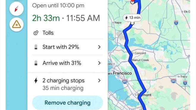
Google, Android Auto temelli elektrikli araçlar için Maps temelli bir şarj güncellemesi yayınladıGoogle, Android Auto işletim sisteminin kullanıldığı tamamen elektrikli araçlar için Maps (Haritalar) temelli bir şarj güncellemesi yayımladı. “Google Maps’in elektrikli araç şarjına yönelik yapay zeka destekli özelliklerini Android Auto temelli 350’den fazla araç modeline getiriyoruz.” diyen Google, bu konuda yaptığı resmi açıklamada, “Artık Haritalar, elektrikli araç modelinize ve batarya doluluk oranınıza göre ne zaman ve nerede şarj etmeniz gerektiğini söyleyecek; böylece hem yolda kalma korkunuz bitecek hem de farklı uygulamalarla uğraşmak zorunda kalmayacaksınız.” ifadelerine yer verdi. 15’ten fazla markaya ait yüzlerce elektrikli araç modeline açılan altyapı, ilk olarak ABD’de sunuluyor. “Yüzlerce aracın batarya tüketimini doğru tahmin edebilmek adına yapay zekayı gelişmiş enerji modelleriyle birleştiriyoruz. Bu modeller; aracın ağırlığı ve batarya boyutu gibi teknik özelliklerin yanı sıra haritalardan gelen trafik, yol eğimi ve hava durumu gibi gerçek zamanlı verileri de analiz ediyor.” diyen Google, sistemi önümüzdeki dönemde küresel olarak da kullanıma alabilir.

Google, Android Auto temelli elektrikli araçlar için Maps temelli bir şarj güncellemesi yayımladı yazısı ilk olarak Teknoloji haberleri – LOG üzerinde yayınlandı.

Microsoft 365 Copilot’un Researcher aracı “Critique” ve “Council” özellikleriyle güçlendirildi

Microsoft 365 Copilot

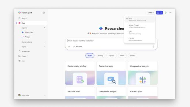
Microsoft 365 Copilot'un Researcher aracı "Critique" özelliğiyle güçlendirildiMicrosoft 365 Copilot’un doğrudan kompleks görevlere odaklanan Researcher aracı, “Critique” ve “Council” adı verilen yeni özelliklerle güçlendirildi. Microsoft CEO’su Satya Nadella tarafından yapılan paylaşıma göre yeni çok modelli derin araştırma sistemi Critique, birden fazla yapay zeka modelinin (GPT ve Claude) bir arada çalıştırılarak olabilecek en ideal sonuçların/raporların elde edilmesine aracılık ediyor. Council ise kullanıcıların aynı istem (prompt) üzerinde birden fazla modeli eş zamanlı olarak çalıştırmasına imkan tanıyor. Bu özellik farklı modellerin hangi noktalarda birleştiğini, hangi noktalarda ayrıştığını ve her bir modelin sonuca katkısını gözler önüne seriyor. Introducing Critique, a new multi-model deep research system in M365 Copilot. You can use multiple models together to generate optimal responses and reports. pic.twitter.com/m4RlQmCKzs — Satya Nadella (@satyanadella) March 30, 2026 New in M365 Copilot: Council. You can run multiple models on the same prompt at the same time, so you can see where they align and diverge, and understand what each adds. pic.twitter.com/2p7O14OLFp […]

Microsoft 365 Copilot’un Researcher aracı “Critique” ve “Council” özellikleriyle güçlendirildi yazısı ilk olarak Teknoloji haberleri – LOG üzerinde yayınlandı.

Building a Face Authentication System for Linux (Using PAM, systemd, and ONNX)

GitHub logo

Linux still lacks a reliable, native biometric authentication system.

While platforms like Windows and macOS have tightly integrated face authentication, Linux users typically rely on passwords — or experimental tools that often break under real-world conditions.

I wanted something:

  • fully offline
  • predictable under PAM
  • extensible and debuggable

So I built AstraLock.

GitHub logo

shekh-2810
/
AstraLock

AstraLock is a lightweight face-authentication system designed for Linux. It replaces legacy camera pipelines with modern deep-learning models, optimized preprocessing, and a clean, modular architecture. The goal is simple: reliable face-based login on Linux without the sluggishness, low-light failures, or angle sensitivity seen in older tools.

AstraLock

AstraLock is a Linux biometric authentication system that enables face-based login through PAM and systemd, designed to be offline, auditable, and hackable, offering a native Linux alternative to projects like Howdy and closed platforms such as Windows Hello without cloud dependencies.

It runs a local daemon that performs facial verification and integrates directly with system authentication flows such as sudo, login, display managers, and polkit.

AstraLock banner

What AstraLock Is

  • A system daemon that performs face verification

  • A PAM module (pam_facelock.so) for system authentication

  • A CLI tool for enrollment, verification, and testing

  • A local-only LBPH model (no cloud, no network)

No external services.
No telemetry.
No vendor lock-in.

Features

  • 🔐PAM authentication (login, sudo, polkit, display managers)
  • 🧠Offline facial recognition (LBPH, OpenCV)
  • ⚙️systemd-managed daemon lifecycle
  • 📷 Webcam support via OpenCV
  • 🧪Built-in testing via pamtester
  • Simple CLI for users and admins

Architecture

…

The Problem with Existing Approaches

Most existing solutions (like Howdy) work — until they don’t.

Common issues:

  • PAM inconsistencies across sudo, login, and display managers
  • unreliable camera handling
  • fragile integration with system components
  • limited control over the authentication pipeline

The biggest issue wasn’t the ML part — it was system integration.

Design Goals

Before writing code, I defined strict constraints:

  • No cloud dependencies
  • No telemetry
  • Deterministic PAM behavior
  • Clean separation between authentication logic and ML
  • Works across CLI and GUI authentication flows

High-Level Architecture

Instead of embedding everything inside PAM, I separated concerns:

Application (sudo / login / GUI)
        ↓
       PAM
        ↓
pam_facelock.so
        ↓
facelockd (systemd service)
        ↓
UNIX socket IPC
        ↓
Face recognition pipeline

Why this design?

PAM modules should stay minimal and predictable.

Heavy operations like:

  • camera access
  • model inference
  • image processing

are handled by a separate daemon.

This avoids blocking PAM and improves reliability.

Recognition Pipeline

The pipeline uses modern ONNX-based models:

  1. Face detection (RetinaFace)
  2. Face alignment (landmark-based)
  3. Embedding generation (ArcFace, 512-dim)
  4. Cosine similarity for matching

Everything runs locally.

No external APIs. No network calls.

Key Challenges

1. PAM Behavior is Subtle

The biggest issue was handling:

  • auth sufficient vs required
  • fallback to password authentication
  • inconsistent behavior across services

Small changes in PAM configuration can completely change outcomes.

2. Display Managers Are Inconsistent

GDM, SDDM, and others:

  • handle authentication differently
  • sometimes retry unexpectedly
  • may break assumptions about flow

This required testing across environments.

3. Camera Reliability

Accessing /dev/video* sounds simple — but:

  • permissions vary
  • devices differ
  • latency can affect authentication timing

4. Avoiding Lockouts

Biometric authentication is probabilistic.

So:

  • password fallback is always preserved
  • PAM is configured as sufficient, not exclusive

Current Capabilities

  • Works with sudo, login, and GUI prompts (polkit)
  • Fully offline inference
  • Local model storage per user
  • systemd-managed daemon
  • CLI for enrollment and verification

Security Considerations

This is not meant to replace passwords entirely.

Important points:

  • biometric matching is probabilistic
  • spoofing is a real concern
  • fallback authentication is required

The system is designed for:

convenience + controlled risk, not absolute security

What I Learned

  • System integration is harder than ML
  • PAM is powerful but unforgiving
  • Reliability matters more than accuracy
  • Simplicity in design reduces failure cases

Looking for Feedback

I’m particularly interested in input on:

  • PAM edge cases in real-world deployments
  • failure modes I might be missing
  • biometric authentication tradeoffs on Linux
  • ways to improve reliability without sacrificing usability

Project

AstraLock is open source and still evolving.

If you’ve worked with PAM, Linux auth, or system-level tooling, I’d appreciate your perspective.

Stop Scraping Bayut – Build a Dubai Property App in 48 Hours

Your Bayut scraper just broke again.

They updated their HTML. Your regex is wrong. The IP got blocked. You’re debugging at midnight instead of shipping.

Sound familiar?

I’ve been there. I built a scraper for Dubai property data. It worked for two months. Then Bayut updated their site. I spent a week fixing it. Then it broke again.

That’s when I found a better way.

The Problem with Scraping Bayut

Web scraping Bayut is painful for a few specific reasons:

  1. Aggressive bot detection – Bayut uses Cloudflare and fingerprinting. Your scraper gets blocked fast.
  2. Frequent HTML changes – The site structure changes regularly. Your selectors break.
  3. Proxy costs – To scrape at scale, you need rotating proxies. That’s $200-500/month minimum.
  4. Legal grey area – Scraping violates Bayut’s terms of service. It’s a real risk.
  5. Maintenance hell – Every site update means debugging time. Time you could spend building.

The Solution: Bayut API

The Bayut API on RapidAPI gives you programmatic access to Bayut’s data without any of those problems.

  • No proxies needed
  • No scraping
  • Clean JSON responses
  • UAE-wide coverage
  • Fast (sub-400ms)

Here’s what you can access:

  • Property listings (sale + rent)
  • Off-plan development projects
  • Agent profiles and listings
  • Agency data
  • Transaction history
  • Location search and IDs

Building the App: Step by Step

Let’s build a Dubai property search app. I’ll use Node.js and Express for the backend.

Step 1: Get Your API Key

Sign up on RapidAPI and subscribe to the Bayut API:

https://rapidapi.com/happyendpoint/api/bayut14/

Step 2: Location Search

First, implement location autocomplete so users can search by area.

const axios = require('axios');

async function searchLocations(query) {
  const response = await axios.get(
    'https://bayut14.p.rapidapi.com/autocomplete',
    {
      params: { query, langs: 'en' },
      headers: {
        'x-rapidapi-host': 'bayut14.p.rapidapi.com',
        'x-rapidapi-key': process.env.RAPIDAPI_KEY
      }
    }
  );
  return response.data.data.locations;
}

// Returns: [{ id, externalID, name, slug, adCount }]
// Use externalID for property search

Step 3: Property Search

Now the core search functionality:

async function searchProperties(params) {
  const response = await axios.get(
    'https://bayut14.p.rapidapi.com/search-property',
    {
      params: {
        purpose: params.purpose || 'for-sale',
        location_ids: params.locationId,
        property_type: params.type || 'apartments',
        rooms: params.bedrooms,
        price_min: params.minPrice,
        price_max: params.maxPrice,
        sort_order: 'popular',
        page: params.page || 1,
        langs: 'en'
      },
      headers: {
        'x-rapidapi-host': 'bayut14.p.rapidapi.com',
        'x-rapidapi-key': process.env.RAPIDAPI_KEY
      }
    }
  );

  const { properties, total, totalPages } = response.data.data;
  return { properties, total, totalPages };
}

Each property in the response includes:

  • Title, price, bedrooms, bathrooms
  • Area in sqm
  • Location details
  • Cover photo
  • Agent info
  • Amenities
  • Completion status (ready vs off-plan)

Step 4: Property Details

When a user clicks a listing, fetch full details:

async function getPropertyDetails(externalId) {
  const response = await axios.get(
    'https://bayut14.p.rapidapi.com/property-details',
    {
      params: { external_id: externalId, langs: 'en' },
      headers: {
        'x-rapidapi-host': 'bayut14.p.rapidapi.com',
        'x-rapidapi-key': process.env.RAPIDAPI_KEY
      }
    }
  );
  return response.data.data;
}

Step 5: Off-Plan Projects

Add a section for new developments:

async function searchOffPlan(locationId) {
  const response = await axios.get(
    'https://bayut14.p.rapidapi.com/search-new-projects',
    {
      params: {
        location_ids: locationId,
        property_type: 'residential',
        sort_order: 'latest',
        page: 1
      },
      headers: {
        'x-rapidapi-host': 'bayut14.p.rapidapi.com',
        'x-rapidapi-key': process.env.RAPIDAPI_KEY
      }
    }
  );
  return response.data.data.properties;
}

What I Built in 48 Hours

Using this API, I built a working property search app with:

  • Location autocomplete (powered by /autocomplete)
  • Property search with filters (powered by /search-property)
  • Property detail pages (powered by /property-details)
  • Off-plan project listings (powered by /search-new-projects)
  • Agent profiles (powered by /agent-details)

Total development time: 48 hours.

With a scraper, this would have taken 3-4 weeks – and it would break every month.

The Numbers

Scraper Bayut API
Setup time 3-4 weeks 2 days
Monthly cost $300-500 (proxies) $10-50
Uptime ~70% 99.9%
Maintenance 10+ hrs/month 0 hrs/month
Legal risk High None

What to Build Next

Once you have the basics working, here are some features to add:

  • Price alerts – notify users when a property drops in price
  • Saved searches – let users save their filters
  • Market analytics – use /transactions to show price trends
  • Agent comparison – rank agents by listing count and area

Get Started

The Bayut API is available on RapidAPI with a free plan:

🔗 https://rapidapi.com/happyendpoint/api/bayut14/

Full documentation:

📖 https://bayutapi.dev/

Questions? Reach out: [email protected]

Built by Happy Endpoint – developer-friendly APIs for real-world data.

🌐 https://happyendpoint.com | 🐦 https://x.com/happyendpointhq

Inside AIO Sandbox (Part 1): Files & Shell — The Foundations of Agent Execution

Modern AI agents are no longer just generating text—they are expected to write files, modify code, and execute commands.
But doing this directly on your local machine or production systems is risky and hard to control.
This is where AIO Sandbox comes in.
It provides an isolated, programmable environment where agents can safely:

  • create and manipulate files

  • run shell commands

  • execute code

  • produce artifacts

In this first post, we’ll focus on the two most fundamental capabilities:

🧩 Filesystem (state)
⚙️ Shell (execution)

By the end, you’ll see how these combine into a complete runtime for agents.

🌐 Multi-language SDK Support

While this tutorial uses Python, AIO Sandbox is not limited to Python developers.
The agent-sandbox SDK also supports:

  • TypeScript / JavaScript

  • Go (Golang)

👉 This makes it easy to integrate AIO Sandbox into a wide range of agent frameworks, backend services, and developer stacks.

🛠️ Prerequisites

  • Python 3.12+

  • A running AIO Sandbox instance at http://localhost:8080

  • Python SDK installed

pip install agent-sandbox

🧠 Mental Model

Think of AIO Sandbox as a remote, disposable Linux machine that your agent controls via APIs.

  • Filesystem → where data and artifacts live

  • Shell → how actions are executed

Simple Flow:
Agent → API → Sandbox → Filesystem + Shell

📁 Part 1 — Working with Files

Let’s start by treating the sandbox like a filesystem.

1.Hello Sandbox Files

Goal: introduce write_file, read_file, and list_path.

from agent_sandbox import Sandbox

client = Sandbox(base_url="http://localhost:8080")

home_dir = client.sandbox.get_context().home_dir

notes_file = f"{home_dir}/hello.txt"

# Write a text file
write_result = client.file.write_file(
    file=notes_file,
    content="Hello from AIO Sandbox!nThis file lives inside the sandbox.",
)

print("Wrote bytes:", getattr(write_result.data, "bytes_written", None))

# Read it back
read_result = client.file.read_file(file=notes_file)
print("File content:")
print(read_result.data.content)

# List files in the sandbox home directory
list_result = client.file.list_path(
    path=home_dir,
    include_size=True,
    sort_by="name",
)

items_to_list = getattr(list_result.data, 'files', getattr(list_result.data, 'entries', []))

for item in items_to_list:
    print(f"- {item.path} ({getattr(item, 'size', 'unknown')} bytes)")

2.Edit a Config File

Goal: show replace_in_file and search_in_file.
💡 Agents often follow a loop:

modify → verify → proceed

from agent_sandbox import Sandbox

client = Sandbox(base_url="http://localhost:8080")

home_dir = client.sandbox.get_context().home_dir
config_file = f"{home_dir}/app.env"

# Create a simple config file
client.file.write_file(
    file=config_file,
    content="MODE=devnPORT=8000nDEBUG=truen",
)

# Replace one value
client.file.replace_in_file(
    file=config_file,
    old_str="MODE=dev",
    new_str="MODE=prod",
)

# Search to verify
search_result = client.file.search_in_file(
    file=config_file,
    regex=r"MODE=.*",
)

print("Search result:")
print(search_result)

# Read final content
final_file = client.file.read_file(file=config_file)
print("nUpdated config:")
print(final_file.data.content)

3.Write and Export an Artifact

Goal: show download_file.

  • sandbox outputs can be streamed out cleanly

  • useful for logs, reports, generated code, screenshots, notebooks, datasets

home_dir = client.sandbox.get_context().home_dir
report_file = f"{home_dir}/report.txt"

# Create an artifact inside the sandbox
client.file.write_file(
    file=report_file,
    content="Run completenStatus: successnArtifacts generated: 1n",
)

# Download it from the sandbox to the local machine
with open("downloaded_report.txt", "wb") as f:
    for chunk in client.file.download_file(path=report_file):
        f.write(chunk)

print("Downloaded sandbox artifact to ./downloaded_report.txt")

4.Discover files

result = client.file.find_files(
    path=home_dir,
    glob="*.txt",
)

print(result)

⚙️ Part 2 — Executing Commands (Shell)

Now let’s make the sandbox do work.

⚠️ Important Notes

  • Shell commands must be passed as keyword arguments:
exec_command(command="...")
  • Output is available at:
result.data.output
  • Exit status:
result.data.exit_code

1. Basic shell command execution (Hello World)

from agent_sandbox import Sandbox

client = Sandbox(base_url="http://localhost:8080")

result = client.shell.exec_command(
    command="echo 'Hello from sandbox shell'"
)

print("Output:", result.data.output)
print("Exit code:", result.data.exit_code)

2. Inspect the sandbox environment

result = client.shell.exec_command(command="pwd")
print("PWD:", result.data.output)

result = client.shell.exec_command(command="ls -la")
print(result.data.output)

👉 The sandbox behaves like a real Linux environment.

3. Execute a Python script

home_dir = client.sandbox.get_context().home_dir
script_path = f"{home_dir}/hello.py"

client.file.write_file(
    file=script_path,
    content="""
print("Running inside sandbox")
print("Computation:", 10 * 5)
""",
)

result = client.shell.exec_command(
    command=f"python3 {script_path}"
)

print(result.data.output)

🔥 This is an important pattern:

Agent writes code → executes it → observes output

4. Install and use a package

# Install package
client.shell.exec_command(command="pip install requests")

# Verify installation
result = client.shell.exec_command(
    command='python3 -c "import requests; print(requests.__version__)"'
)

print("Requests version:", result.data.output)

💡 Shows:

  • sandbox is mutable

  • supports dynamic dependencies

5. Chain commands

result = client.shell.exec_command(
    command="mkdir -p demo && echo 'hello' > demo/file.txt && cat demo/file.txt"
)

print(result.data.output)

6. Check exit codes

result = client.shell.exec_command(command="ls non_existent_file")

print("Output:", result.data.output)
print("Exit code:", result.data.exit_code)

Agents should check exit codes, not just output.

🧩 Bringing It Together

At this point, we’ve seen:

Filesystem (state)

Core primitives to showcase:

  • create

  • read

  • modify

  • search

  • list

  • discover

Shell (execution)

Core primitives to showcase:

  • run commands

  • execute scripts

  • inspect environment

🎯 Key Insight

AIO Sandbox gives agents a safe, programmable runtime:

  • Files → memory/state

  • Shell → actions

Together, they enable real-world workflows like:

  • code generation and execution

  • data processing

  • automation pipelines

  • tool orchestration

🚀 What’s Next

Thanks for reading! Hope it was helpful! This is just the beginning. In upcoming posts, we’ll dive into topics such as:

  • 🌐 Browser automation (CDP-based)

  • 🔌 MCP tool integration

  • 📓 Jupyter / notebook execution

  • 🤖 OpenClaw integration

  • 🎯 Reinforcement learning inside sandbox

💬 Final Thoughts

AIO Sandbox bridges the gap between:

  • “LLM that generates text”

  • and

  • “Agent that can actually do things”

And it does so safely, reproducibly, and programmatically.

Open Tables, Shared Truth: Architecting a Multi-Engine Lakehouse

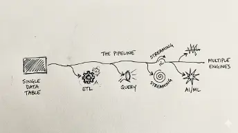
In the modern data landscape, we often hear the phrase “single source of truth.” But as many data engineers know, the reality behind that phrase is often a complex web of data copies, inconsistent metrics, and redundant governance.

The problem isn’t processing data. It’s where truth lives.

For over a decade, we’ve been solving the wrong problem in data engineering.

We’ve optimized compute. We’ve scaled storage. We’ve built faster pipelines.

And yet—
we still don’t trust our data.

This blog is not about introducing another analytics engine or tool. It’s about challenging a design flaw we’ve collectively normalized—and showing how modern lakehouse architectures are finally fixing it.

The Problem We Stopped Questioning

Let’s start with an uncomfortable truth.Most organizations today have:

  • The same dataset copied multiple times
  • The same metric producing different results
  • Governance logic re-implemented across systems

And yet, we confidently say:

“We have a single source of truth.”

But do we really?

In reality, what we have is:

  • A warehouse copy
  • A lake copy
  • A serving copy

Each slightly different. Each “correct” in its own context.

From Data Copies to Data Contracts

Why did we end up here? Because historically:

  • Compute engines couldn’t agree on formats
  • Storage systems lacked transactional guarantees
  • Governance was tied to specific platforms

So we did what engineers do best:
👉 We built pipelines. Lots of them.

Pipelines became the glue holding together fragmented truth. But pipelines don’t scale truth — they multiply it.

Why “Querying the Lake” Wasn’t Enough

The industry tried to fix this with data lakes. We said:

“Let’s store everything in one place”
“Let’s allow multiple engines to query it”

And yes, we achieved:

  • Faster access
  • Fewer ETL jobs
  • Flexible analytics

But we missed something critical:

Ownership didn’t change.

The lake became accessible—but not authoritative.

The Real Shift: From Engines → Tables

Here’s the mindset shift that changes everything:

The unit of ownership is not the engine. It’s the table.

Historically:

  • Engines owned data
  • Pipelines moved data between engines

Now:

  • Tables become shared, governed, authoritative assets

This is where open table formats like Apache Iceberg, Delta Lake, and Apache Hudi come in.

What Makes Open Tables Different?

Open table formats bring database-like guarantees to object storage:

  • ACID transactions
  • Schema evolution
  • Time travel
  • Snapshot isolation
  • Concurrent reads and writes

But the real magic is this:

👉 Multiple engines can read and write to the same table reliably

Engines like:

  • Apache Spark
  • Trino
  • Amazon Athena
  • Snowflake

…can all operate on the same dataset.

No duplication. No translation layers.

Writing Back to the Lake

This is where things truly evolve.

In traditional architectures:

  • Transformations write to new systems
  • Each system maintains its own “truth”

In a modern lakehouse:

  • Transformations write back to shared tables
  • These tables become data products

👉 The lake is no longer just storage. It’s the system of record.

Where Control Actually Lives?

Another critical shift:

Governance moves from engines → to the table layer

Instead of duplicating policies across systems, you define them once:

  • Access controls
  • Column-level security
  • Schema ownership
  • Audit trails

Technologies like AWS Lake Formation enable centralized governance across engines.

Now:

  • Engines come and go
  • Policies stay consistent

The Reference Architecture: Multi-Engine Lakehouse

A modern architecture looks like this:

  1. Storage Layer: Object storage (e.g., Amazon S3)
  2. Table Layer: Open table formats (Iceberg/Delta/Hudi)
  3. Compute Layer: Multiple engines (Spark, Trino, Athena, etc.)
  4. Governance Layer: Centralized policy enforcement
  5. Consumption Layer: BI, ML, APIs

And here’s what’s missing:
❌ No “gold copy”
❌ No duplicated datasets
❌ No pipeline sprawl

The Pivot: Two Architectures, Same Problem

Traditional Approach

  • Data is copied
  • Pipelines everywhere
  • Multiple versions of truth

Modern Approach

  • Data is shared
  • Minimal pipelines
  • One consistent truth

Same problem.
Two very different philosophies.

Common Anti-Patterns (That Still Exist)

Even with open tables, teams often fall into traps:

  • Treating tables like CSV files
  • Having no ownership model
  • Allowing every engine to write freely
  • Ignoring cost and compaction strategies

Technology alone doesn’t solve the problem. Design discipline does.

Design Trade-offs You Must Consider

This architecture isn’t “free”.

You need to think about:

  • Concurrent writers → Conflict resolution strategies
  • Compaction ownership → Who maintains table performance?
  • Performance tuning → Partitioning, indexing
  • Failure domains → What breaks, and where?

These are platform decisions—not just engineering ones.

Rethinking Data Ownership

This shift is bigger than technology.

It’s an organizational change.

You move from:

  • Pipeline ownership → Data product ownership
  • System silos → Shared contracts
  • Tool-centric thinking → Agreement-centric thinking

Key Takeaways

  • Stop copying data
  • Start sharing truth
  • Design tables as products
  • Let engines be interchangeable

And most importantly:

“The most scalable analytics platforms are built around agreements, not tools.”

Final Thought

We’ve spent years optimizing how fast we process data.

Now it’s time to ask a better question:

Where does truth live? and who owns it?

Because until that’s solved,
no amount of compute will fix your data platform.

Bad Code Is a High-Interest Loan: How Technical Debt Slowly Kills Team Velocity

We were moving fast.

Features shipped every week.

Stakeholders were happy.

The backlog was finally under control.

Then, almost without noticing, everything slowed down. A feature that should have taken a day took three abd a small change broke something unrelated. Fixing bugs started taking longer than building new features.
And at some point, someone said:

“But this used to be faster, right?”

They weren’t wrong. At some point in the past, things were faster, but that speed came at a cost.

A cost that wasn’t visible at the time.
A cost that quietly accumulated.

This is something I’ve often wanted to explain to non-technical stakeholders:

we didn’t suddenly become slower, we’re just paying back what we borrowed.

TL;DR

  • Technical debt behaves like a high-interest loan: it feels cheap at first, but becomes expensive over time.
  • The real problem isn’t having technical debt, it’s letting it compound unmanaged.
  • Refactoring isn’t a cost, it’s an investment with measurable ROI in team velocity.

Table of Contents

  • The Illusion of Speed
  • Technical Debt as a Financial Model
  • Where the Interest Shows Up
  • The Compounding Effect
  • When Teams Hit Default
  • The ROI of Refactoring
  • When NOT to Refactor
  • Practical Ways to Manage Technical Debt
  • Final Thoughts

The Illusion of Speed

Technical debt often starts as a conscious trade-off:

  • You skip a refactor.
  • You duplicate a bit of logic.
  • You hardcode something “just for now”.

And in the moment, it feels like the right decision because:

  • You move faster.
  • You deliver sooner.
  • You hit the deadline.

That’s why it’s so hard to avoid, because it works, but what you’re really doing is borrowing time from your future self and like any loan, that time comes back.

Technical Debt as a Financial Model

One of the most useful ways to think about technical debt is to treat it like an actual financial system.
Not just a metaphor, but a model.

Principal: the shortcut

The principal is the initial shortcut you take:

  • skipping a proper abstraction
  • duplicating logic instead of extracting it
  • shipping a workaround instead of fixing the root cause

Individually, these decisions are often reasonable.

Sometimes even necessary.

Interest: the friction

The interest is what you pay every time you touch that code again. It shows up as:

  • extra time to understand what’s happening
  • unexpected side effects
  • more effort to implement even simple changes

You don’t notice it immediately.

But it’s there, every time.

Compounding: the multiplier

And then comes the real problem: compounding.

Each new feature built on top of messy code increases the cost of the next one.

Not linearly.

Exponentially.

Where the Interest Shows Up

Interest doesn’t arrive as a big, visible cost, it shows up as friction.

Small things that make your work just a bit slower, every single day.

  • A feature takes longer than expected
  • A bug fix introduces another bug
  • You spend more time reading code than writing it
  • Onboarding a new developer becomes difficult

Or even something like this:

// "temporary" workaround from 6 months ago
if (user.role === "admin" && featureFlagX) {
  // special case inside special case
}

Nothing here breaks the system, but everything here slows you down.

That’s the interest you’re paying.

The Compounding Effect

This is where things become dangerous.

Technical debt doesn’t just add cost, it multiplies it. Every new feature built on top of unclear or fragile code becomes:

  • harder to implement
  • harder to test
  • harder to change

So the next feature takes longer.

And the next one.

And the next one.

At some point, the system isn’t just complex.

It’s actively resisting change.

And that’s when velocity starts dropping, even if your team hasn’t changed at all.

When Teams Hit Default

In finance, default happens when you can’t repay your debt anymore.

In software, it looks different, but the signal is clear.

You see it when:

  • refactoring is always postponed
  • certain parts of the codebase are avoided
  • every release feels risky
  • progress slows down despite increasing effort

At this stage, teams often react the wrong way.

They try to push harder.

More hours.

More pressure.

More “just ship it”.

But the problem isn’t effort.

It’s accumulated complexity.

And no amount of speed can compensate for that.

The ROI of Refactoring

Refactoring is often perceived as a cost, something that slows down delivery, something you “don’t have time for”, but that perspective ignores the return.

Refactoring is an investment.

And like any investment, it pays off over time.

Let’s make it concrete, imagine:

  • A feature currently takes 3 days to implement
  • After refactoring, similar features take 1.5 days

That’s a 50% improvement.
Over 10 features, you’ve saved 15 days.
That’s not just cleaner code, that’s recovered velocity.

And just like debt compounds negatively, good code compounds positively:

  • faster development
  • fewer bugs
  • easier onboarding
  • more confidence in changes

This is where engineering meets business, because velocity is not just a technical metric, it’s a business advantage.

When NOT to Refactor

Not all debt needs to be repaid immediately, and not all code needs to be perfect.

Refactoring everything blindly can be just as harmful.

Avoid refactoring when:

  • the code is rarely touched
  • the feature is about to be replaced
  • you’re still validating a product idea
  • the cost clearly outweighs the benefit

The goal is not to eliminate technical debt, but it’s to manage it intentionally.

Practical Ways to Manage Technical Debt

You don’t need a full rewrite to stay in control, you need consistency.

A few habits make a huge difference over time:

  • Refactor as you go: improve code while you’re already working on it
  • Make debt visible: track it instead of hiding it
  • Set a refactoring budget: even 10–20% of time is enough
  • Review for maintainability, not just correctness
  • Call out complexity early, before it spreads

These are small actions, but they prevent large problems.

Final Thoughts

Technical debt isn’t the enemy, it’s a tool.

Sometimes you take on debt to move faster and that’s a valid decision, but if you ignore it, it becomes a liability and, eventually, it starts slowing everything down.

The real problem isn’t having technical debt.

It’s pretending you don’t.

If this resonated with you:

  • Leave a ❤️ reaction
  • Drop a 🦄 unicorn
  • Share the most “expensive” piece of bad code you’ve seen

And if you enjoy this kind of content, follow me here on DEV for more.

Weather MCP

  • Background
  • Result
  • Learning

TODO Add other headers

Background

During my career break that I started in 2025, I started exploring the ever-changing Generative AI landscape. In Decemember, I was exploring Spring Boot as I hadn’t used it in anger professionally having used other Java frameworks like Jersey, Play and I wanted to build something.

In February, everyone in the UK was talking about how it had rained everyday in 2026 so far. I thought that generative AI chatbots like our friend ChatGPT shouldn’t miss out on the conversation.

So I set out to build a Model Context Protocol (MCP) server using Spring AI and developed using Cursor agents.

3 things I could tick off my tech backlog (which is probably just as long as my gaming backlog).

Result

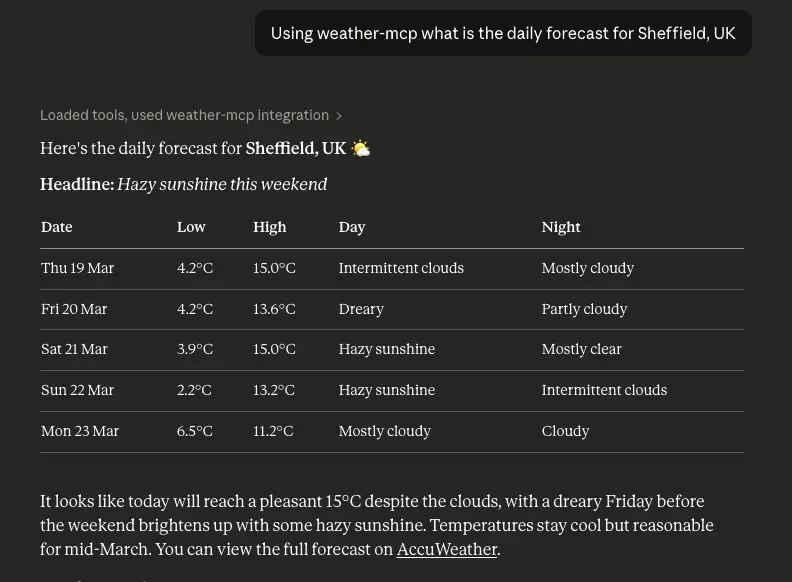
An Accuweather MCP server that provides prompts and tools for agents to be able to find out for a location:

  • The current weather
  • Hourly forecast
  • Daily forecast

This is available on the official MCP Registry

Here’s what it looks like integrated within Claude:

I had fun building this out and thought I would wrap it up by creating this post, sharing the resources I used to learn as well as gotchas I encountered. Hopefully not only useful for future Jonathan, but others too 😀

Learning

You will see a pattern here, but it’s how I prefer to learn (I appreciate others may prefer to watch paint dry)

Cursor

Cursor themselves provide great resources that includes plenty of guidance, recommendations and best practises.

Model Context Protocol

If you want to get started and get to grips with the Model Context Protocol, the official documentation is great.

I even encourage anyone to read the specification as for servers it details error handling, implementation considerations and security.

Spring AI

The Spring AI reference provides plenty of guidance and recommendations around MCP as well as other parts of Genative AI such as using chat clients or RAG.

One especially helpful resource were the Spring AI examples that showcase putting everything together. For example, how to use the MCP annotations to create MCP tools.

Gotchas

Time for something more interesting, below are things that I encountered whilst building out my MCP server that took a minute to resolve and more likely help the next person.

Cursor – agents

My goal of this side project was to get used to Agentic development and minimise hand-rolling code. When I started out with a blank slate and aimed to build the current weather feature, I tried one-shotting it by generating a plan and seeing what the result was. Although it did the job, the Agent produced a lot of code to review and used patterns that I didn’t want to use. So I then had to course correct with more prompts.

A lot of this is in the Cursor docs, but here’s how I improved things for the next feature:

  • Added guard rails: Added unit and integration tests, added auto code formatting with spotless, added code analysis using checkstyle
  • Incremental rule creation: Any time an Agent got something wrong e.g. it tried to use maven to run a Gradle project, it didn’t denote nullables using JSpecify; I added a rule to AGENTS.md
  • Use Plan mode and auto model selection: I used Plan mode to define what I wanted and let Cursor decide on which model to use (this helped stretch the Hobby plan as far as I could before purchasing a Pro plan)
  • Develop in increments: Instead of building out the daily forecast feature in one go, I got the Agent to build it out layer by layager (HTTP Client, Gateway and MCP Tool). That way I had less code to review and can course correct easier.
  • Reference examples: Once I didn’t have a blank slate anymore, I referenced existing code as examples so the Agent knew what patterns to follow.

By doing all of this, when it came to the hourly forecast feature, I delegated the entire thing to a Cloud Agent and only had to review the changes.

Spring AI

  • turn off console logging
  • Debugging using with mcp inspector or claude
  • using mcp annotations

MCP registry

  • use validate to confirm e.g. description length
  • docker version number at end

Publishing

  • use jib over semantic release plugins to support multi-arch images

Right-Sizing vs. Auto-Scaling: Which Saves More on EKS?

Right-Sizing vs. Auto-Scaling: Which Saves More on EKS?

Most EKS cost conversations end up in the same place: someone enables Cluster Autoscaler, watches the node count drop slightly, and calls it done. Then the bill barely moves. The reason is that Cluster Autoscaler and right-sizing solve different problems, and applying one without the other leaves most of the savings on the table.

This piece breaks down what each approach actually does, where each wins, and in what order to apply them.

The Billing Model That Makes Right-Sizing So Powerful

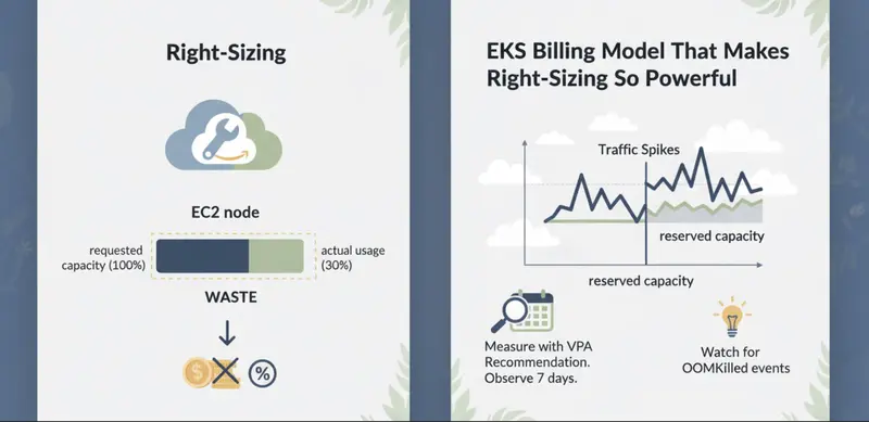
EKS bills for EC2 node capacity, not for what your pods consume. A node is running, so you pay for it, regardless of whether pods use 10% or 90% of its resources.

The waste happens at the request level. Kubernetes uses resource requests, not actual usage, to schedule pods onto nodes. When a pod requests 2 vCPU and uses 0.3 vCPU in practice, that 1.7 vCPU is reserved and unavailable for any other workload. The node fills up on paper while sitting mostly idle in practice.

At $0.384/hr for an m5.2xlarge in us-east-1, that cluster pays for 8 vCPU per node but gets meaningful work out of fewer than 3. Cluster Autoscaler cannot fix this. It sees the node as utilized because requests are high. It will not remove the node even though actual usage is low.

Right-sizing corrects the requests. Once requests reflect real usage, nodes can fit more pods, fewer nodes are needed, and Cluster Autoscaler can actually remove underutilized nodes.

What Right-Sizing Actually Changes

Right-sizing has two layers on EKS: pod-level requests and node-level instance sizing.

At the pod level, the goal is to set CPU and memory requests close to the 90th-percentile actual usage, not at a round number someone picked during deployment. The Vertical Pod Autoscaler (VPA) in Recommendation mode observes pod metrics over time and produces a suggested request value. It does not apply the change automatically in Recommendation mode. You review and apply it yourself.

The impact compounds quickly. Consider a service running 10 replicas on an m5.2xlarge cluster:

Metric Before Right-Sizing After Right-Sizing
CPU request per pod 1000m 250m
Memory request per pod 2 GB 512 MB
Pods per node (bin-packing) 4 14
Nodes needed for 10 replicas 3 1
On-demand hourly cost (us-east-1) $1.15 $0.384
Monthly cost (730 hrs) $840 $280

The 10 replicas did not change. The pods do the same work. The only thing that changed is what the pods told Kubernetes they needed. That correction removed two nodes permanently.

At the node level, right-sizing means choosing instance types that match the actual pod profile of the workload. A cluster running memory-light, CPU-bound services wastes money on r5 instances. Moving to c5 instances gives more vCPU per dollar. AWS Compute Optimizer analyzes CloudWatch metrics from your managed node groups and recommends instance type changes. It is free to run.

Right-sizing is a one-time correction with a permanent effect on your baseline bill.

How Auto-Scaling Addresses a Different Problem

Auto-scaling does not reduce per-pod waste. It matches the number of running pods and nodes to current demand, which is a different problem entirely.

Horizontal Pod Autoscaler (HPA) adds or removes pod replicas based on CPU utilization or custom metrics. When traffic spikes, more pods appear. When traffic drops, excess pods terminate. This prevents the cluster from being statically sized for peak load when average load is much lower.

Cluster Autoscaler works at the node level. When pending pods cannot be scheduled because no node has enough capacity, it provisions a new node. When a node’s actual utilization drops below a threshold for 10 consecutive minutes, it removes it. The trigger is pod requests, not actual CPU or memory usage.

KEDA extends HPA with event-driven scaling. Instead of scaling on CPU, you can scale on queue depth, Prometheus metrics, scheduled time windows, or external signals. A batch processor that runs overnight can scale to zero during business hours and scale back up at midnight.

Auto-scaling is most valuable when the load is genuinely variable. A service that gets 5x more traffic at noon than at midnight should not run peak-capacity nodes all day. Auto-scaling handles that. A service that runs at steady load 24 hours a day gets nothing from HPA, but gets real savings from right-sizing.

The critical failure mode: if you enable HPA on overprovisioned pods, every new replica inherits the bloated requests. Scaling from 5 pods to 15 pods triples the cluster cost, but the actual work is the same per replica, just distributed across more instances.

Where Each Approach Wins and Where It Fails

Dimension Right-Sizing Auto-Scaling
Traffic pattern Steady or predictable load Variable, spiky, or event-driven load
Type of savings Reduces baseline cost permanently Reduces cost during off-peak periods
Engineering effort One-time: measure, apply, verify Ongoing: tune thresholds, monitor lag
Time to value 1 to 2 weeks of VPA observation Hours to configure, tuning takes weeks
Primary failure mode Pods OOMKilled if requests set too low HPA lag during sudden traffic spikes
Best tool VPA Recommendation + Compute Optimizer HPA + Cluster Autoscaler + KEDA

Right-sizing delivers immediate, permanent reduction. It works regardless of traffic shape because it corrects the structural waste in how pods claim resources. Auto-scaling delivers proportional reduction on variable workloads. It works because it removes capacity that is genuinely not needed at a given moment.

Neither approach alone is complete. Right-sizing a statically-sized cluster still leaves it over-provisioned for off-peak hours. Auto-scaling an unright-sized cluster scales up and down efficiently.

The one situation where auto-scaling wins outright: EKS Fargate. Fargate charges per vCPU-second and GB-second of actual pod requests, not for idle node capacity. Right-sizing requests directly reduces the bill with no node management. But Cluster Autoscaler is irrelevant on Fargate since there are no nodes to manage. KEDA and HPA still apply.

The Right Order: Right-Size First, Then Auto-Scale

Applying both approaches in the correct sequence is where the real savings appear. The sequence we use in production:

Step 1: Measure with VPA Recommendation. Deploy VPA in Recommendation mode and let it observe your workloads for at least 7 days. Include a representative sample of traffic, including any weekly peaks. VPA will output a suggested CPU and memory request based on observed percentiles.

Step 2: Apply right-sized requests. Take the VPA recommendation, add 15-20% headroom for burst, and apply it to your pod specs. Roll this out service by service, not all at once. Watch for OOMKilled events in the first 24 hours. An OOMKill means the memory request was set below the actual peak usage. Adjust and re-roll.

Step 3: Tune HPA thresholds. HPA uses CPU target as a percentage of the pod’s CPU request. If a pod requests 1000m CPU and you set HPA to target 70%, it scales at 700m actual CPU. After right-sizing to 250m CPU, that same 70% target triggers at 175m actual CPU. If your workload doesn’t spike that low, HPA will never scale. Recalibrate the target percentage after right-sizing.

Step 4: Validate Cluster Autoscaler behavior. After right-sizing, nodes should consolidate. Cluster Autoscaler should remove nodes that are now underutilized because pods pack more efficiently. If it does not, check the --scale-down-utilization-threshold setting. The default is 50% of requests. With right-sized requests, actual usage should be closer to requests, so utilization will read higher and nodes may survive scale-down review. You may need to lower the threshold slightly or enable bin-packing with the --balance-similar-node-groups flag.

On a 3-node m5.2xlarge cluster running 15 services, this sequence typically consolidates to 1-2 nodes and reduces the hourly EC2 cost from $1.15 to $0.38-0.57. That is a 50-67% reduction. Auto-scaling on its own, without the right-sizing step, would have reduced cost only during off-peak windows, yielding a smaller net monthly reduction.

Right-sizing wins on immediate, permanent impact. Auto-scaling wins on dynamic efficiency. Run both. Run right-sizing first.

Conclusion

If you only auto-scale, you are efficiently managing a wasteful architecture. If you only right-size, you are running a lean architecture that can’t breathe with your traffic.

The most significant EKS savings don’t come from a single “silver bullet” setting; they come from the Right-Size → Bin-Pack → Auto-Scale pipeline. By correcting your pod requests first, you provide the Cluster Autoscaler with the accurate data it needs to actually trigger a scale-down.Start with VPA in recommendation mode today and let your monthly AWS bill reflect the difference.