A few months ago I was trying to sell a second-hand PlayStation. I spent 45 minutes searching eBay, scrolling Facebook Marketplace, trying to figure out if €280 was a fair price or if I was leaving €80 on the table.
That’s a solved problem. It shouldn’t take 45 minutes.
So I built ValueScan — an AI-powered item valuation tool. You describe an item or upload a photo, and it gives you the retail price, resale range, a recommended listing price, and exactly where to sell it. In about 10 seconds.
Here’s what I built it with, what I learned, and where it stands today.

The tech stack
Frontend: React 19 + Vite. Nothing exotic — just a chat interface with a valuation card renderer. The whole UI is one App.jsx file which I probably should have split up but here we are.
AI: Google Gemini 2.5 Flash via a Vercel serverless function. I chose Gemini over GPT-4 for two reasons: vision support for photo uploads is solid, and the cost per token is significantly lower for a use case that generates long structured responses.
The prompt is doing a lot of the work. The AI returns a strict structured format — ITEM:, RETAIL:, RESELL:, SELL:, PLATFORM:, FLIP:, CONFIDENCE: — which I then parse with regex and render into a proper card UI. No JSON, no function calling, just reliable structured text output with a tight system prompt.
Auth + database: Supabase. Email/password auth with hCaptcha, Google OAuth, and a subscriptions table that tracks Pro status. Valuation history is stored per user for Pro subscribers.
Payments: Stripe. €5/month subscription with a webhook that updates Supabase on payment events. The whole checkout flow is one serverless function.
Deployment: Vercel. The API routes live in /api/ and deploy as Edge Functions automatically. Zero config.
PWA + Android: The app is a PWA with a manifest, service worker, and a TWA wrapper for Google Play. So it runs in the browser, installs on desktop, and is listed on Android — same codebase.

The interesting engineering bits
Location-aware pricing. When a user first opens the app, I use the Geolocation API to reverse-geocode their coordinates via Nominatim (OpenStreetMap’s free geocoder). That city + country string gets injected into every Gemini prompt. So a user in Cyprus gets Bazaraki.com and Facebook Marketplace CY suggestions, while a user in Germany gets AutoScout24 and eBay.de. Same model, completely different output.
The scanner. I used html5-qrcode for barcode scanning — point your camera at any barcode and it reads the product, then triggers a valuation automatically. For Pro users only (one free try on the free plan). The scan event gets logged to Supabase with detected item, confidence, and whether a valuation was triggered, which gives me useful data on what people are scanning.
Free limits in localStorage. The free plan is enforced client-side with localStorage counters — message count, image count, scanner uses. Yes, a technically savvy user could clear storage and reset. That’s fine. The people who do that were never going to pay anyway, and it keeps the server completely stateless.

What I got wrong
The README is still the Vite boilerplate. I shipped everything else and forgot to write documentation. If anyone tries to run this locally they’ll have no idea what environment variables to set. Do the README first.
I built the scanner before validating it. The camera-based scanner was the hardest feature to build and it’s the one people use least in testing. I should have validated with text input first and added the scanner later.
No analytics at launch. I have no idea how people are using the app in closed testing because I didn’t add any event tracking. I’m adding Google Analytics now but I’ve already missed two weeks of data.

Where it stands today
Six days into a 14-day closed testing period on Google Play. The app is live at valuescan.app, the Android version is in closed testing, and I’m working through the SEO and marketing foundation before the public launch.
The pricing is €5/month for Pro. The free tier is generous enough to try it properly — 10 messages, 2 image uploads, one free scanner scan.
The niche is real. People genuinely want to know what their stuff is worth before selling. The question “how much is my item worth?” gets searched millions of times a month and there’s no clean, fast, AI-native answer for it yet.

What’s next

Public launch on Google Play (8 days)
Product Hunt launch on the same day
Blog posts targeting specific search queries (“PS5 resale value”, “how much is my iPhone worth”)
Adding more local marketplace awareness — right now it knows about the big ones but I want to expand the local database

If you’re building something in the resale / secondhand space, or you just want to check what something’s worth, give it a try at valuescan.app. Free to start, no card required.
Follow the build:

X / Twitter: @valuescan_ai
Instagram: @valuescan
TikTok: @valuescan

Built by a solo founder in Cyprus. Questions welcome in the comments.

protocol MovieLoader {
    func load() async throws -> [Movie]
}

struct MovieList: View {
    @State var movies = [Movie]()
    let loader: MovieLoader
    var body: some View {
        List(movies, rowContent: MovieRow.init)
            .task { await load() }
    }

    func load() async {
        movies = (try? await loader.load()) ?? []
    }
}

func test_load_loadsMovies() async {
    let expected = [anyMovie()]
    let stubbed = StubMovieLoader(stubs: expected)
    let sut = MovieList(loader: stubbed)
    await sut.load()
    XCTAssertEqual(sut.movies, expected)
}

If you try to run this test as-is, it will fail.

Thehe reason is that @State in a SwiftUI view only connects to an in-memory store if the view has been mounted into a real view hierarchy. The most common workaround is to move the logic into an @Observable.

@Observable class MovieListViewModel {
    var movies = [Movie]()
    let loader: MovieLoader
    init(loader: MovieLoader = RemoteMovieLoader()) { ... }
    func load() async {
        movies = (try? await loader.load()) ?? []
    }
}

struct MovieList: View {
    @State var vm = MovieListViewModel()
    var body: some View {
        List(vm.movies, content: MovieRow.init)
            .task { await vm.load() }
    }
}

func test_load_loadsMovies() async {
    let expected = [anyMovie()]
    let stubbed = StubMovieLoader(stubs: expected)
    let sut = MovieListViewModel(loader: stubbed)
    await sut.load()
    XCTAssertEqual(sut.movies, expected)
}

This pattern, widely used and considered a de facto standard, comes with some drawbacks:

1. We abandon value types purely for the sake of testability.
2. We introduce reference types with all their baggage (lifecycle management and potential leaks) into a framework designed to be as value type-oriented as possible.
3. We keep mixing UI state logic (how and when it updates) with the storage itself, despite introducing an extra object to abstract it — even though stateless MVVM implementations exist even in UIKit.

The solution, curiously, has been in SwiftUI from the start.
In this article I’d like to present an alternative, building on the work of Lazar Otasevic.

Binding

@State is not testable outside a view hierarchy, but @Binding offers a way to expose state for testing — something that seems to have gone largely unnoticed by the community.
Conceptually, a @Binding can be understood as a simple pair of closures (get and set):

struct Binding<Value> {
    let get: () -> Value
    let set: (Value) -> Void
}

Which makes a view using @Binding fully testable:

struct MovieList: View {
    @Binding var movies: [Movie]
    let loader: MovieLoader
    var body: some View {
        List(movies, rowContent: MovieRow.init)
            .task { await load() }
    }

    func load() async {
        movies = (try? await loader.load()) ?? []
    }
}

func test_load_loadsMovies() async {
    var storage = [Movie]()
    let binding = Binding(get: { storage }, set: { storage = $0 })
    let expected = [anyMovie()]
    let stubLoader = StubMovieLoader(stubs: expected)
    let sut = MovieList(movies: binding, loader: stubLoader)
    await sut.load()
    XCTAssertEqual(storage, expected)
}

The view no longer owns its state, becoming a purely functional component that delegates persistence to its ancestor.

SwiftUI is already a state engine; @Binding is simply the wire that lets us connect that engine to our unit tests.

We can build some helper utilities. Analogous to Apple’s static Binding.constant(), we can have a Binding.variable():

extension Binding {
    static func variable(_ initialValue: Value) -> Self {
        var copy = initialValue
        return Binding(get: { copy }, set: { copy = $0 })
    }
}

func test_load_loadsMovies() async {
    let expected = [anyMovie()]
    let stubLoader = StubMovieLoader(stubs: expected)
    let (sut, movies) = makeSUT(loader: stubLoader)
    await sut.load()
    XCTAssertEqual(movies(), expected)
}

func makeSUT(movies: [Movie] = [], loader: MovieLoader) -> (MovieList, () -> [Movie]) {
    let movies = Binding.variable(movies)
    let sut = MovieList(movies: movies, loader: loader)
    return (sut, { movies.wrappedValue })
}

Binding.variable doesn’t create a special container like @State ; it simply captures a local variable via closures. When the view writes:

movies = newValue

…it’s actually executing the set closure, which mutates copy.

And when you read in the test:

movies.wrappedValue

…you’re executing the get closure, which returns that same copy. The view and the test share the same storage, since both use the captured variable.

The view’s state logic is fully testable. Whoever builds it needs to provide it with its state:

import Movies   
import MoviesUI

// Composition Root
struct MovieListComposer: View {
    @State var movies = [Movie]()
    let loader: MovieLoader
    var body: some View {
        MovieList(movies: $movies, loader: loader)
    }
}

We can also create a generic wrapper for views using this pattern:

struct Host<Initial, Content: View>: View {
    typealias Binding = SwiftUI.Binding<Initial>

    @State var state: Initial
    let content: (Binding) -> Content

    init(
        _ state: Initial, 
        @ViewBuilder content: @escaping (Binding) -> Content
    ) {
        self.state = state
        self.content = content
    }
    var body: some View {
        content($state)
    }
}

struct SomeApp: App {
    var body: some Scene {
        WindowGroup {
            Host([Movie]()) {
                MovieList(movies: $0)
            }
        }
    }
}

Conclusions and Considerations

This pattern enables a high level of testability while preserving the simplicity of SwiftUI‘s declarative system, without intermediate layers.

• You don’t need a @observable ViewModel to test state logic in SwiftUI if you don’t need idenitity for your specific use case (most cases).
• @State has storage that is inaccessible outside the SwiftUI runtime. @Binding has no storage of its own and only represents access to external storage via closures.
• By using @Binding, we keep the view as a lightweight, testable struct, without forcing the creation of a class just to satisfy the test runner.
• You can still use @Observable for state, since @Binding is the communication interface, not the storage. This decouples the view from how the data is stored (whether in @State , an @Observable, or a property wrapper from CoreData/SwiftData/etc.).
• Encapsulating logic in a dedicated struct for reuse across views and a more decoupled architecture is entirely possible. For more details, I recommend the the “True Logic: Stateless and Pure” section of this article from Lazar Otasevic. I’ve also published an example project that can serve as a reference: OnlyGoodMovies on how to architecture a project around this design pattern.

How I Replaced Axios With fetch Without Breaking the App

This migration did not happen because I woke up one day and decided to become a minimalist monk of HTTP clients.

It happened because of the Axios compromise story.

According to the Fireship video summary that pushed me to take this seriously, attackers allegedly compromised the project maintainer’s npm account and published malicious Axios versions. Those versions reportedly pulled in a rogue dependency called plain-crypto-js, which is exactly the sort of package name that sounds fake even before it ruins your week.

From the summary, the malicious package used a post-install script as a RAT dropper. It would detect the OS, download a second-stage payload from a command-and-control server, establish remote access, and then clean up after itself to avoid leaving obvious evidence in security audits.

That is an insane sentence to write about a package manager.

So yes, this migration started because of a security concern, but also because npm packages have been losing trust lately in a very “are we serious right now?” kind of way.

So I removed it.

Not in a dramatic, “delete it and pray” kind of way. More in a calm, boring, production-safe kind of way. Which, honestly, is the better kind of dramatic.

Also, sorry Fireship for using your YouTube thumbnail.

Why I Did This Now

The security angle was the whole reason this moved from “nice cleanup idea” to “do it now.”

Based on that Fireship summary, the practical advice was:

• check package.json for the affected Axios versions
• check node_modules for plain-crypto-js
• if compromised, do not just delete the file and move on
• roll API keys and tokens immediately
• follow proper incident cleanup guidance, like the kind Step Security documents

That last part is important. If a machine is compromised, deleting one sketchy package is not a victory lap. That is just the beginning of a worse conversation.

In my case, the safest and cleanest move for the project was simple: remove Axios entirely and replace it with something tiny that I control.

The Goal

I did not want a huge rewrite.

I did not want to touch every API call in the app.

And I definitely did not want to replace Axios with “just raw fetch” and then spend the next two days fixing things that Axios had been quietly doing for me all along.

So the real goal was simple:

Replace Axios with a small internal client built on top of fetch, while keeping the same developer experience for the app.

The Important Realization

A lot of people say, “Why not just use fetch? It already returns promises.”

That part is true.

But Axios was doing a few useful things for us:

• It handled a base URL
• It serialized JSON requests nicely
• It rejected on failed responses
• It let us return response.data directly
• It gave us a clean place to normalize errors

fetch gives you the raw ingredients. Axios gives you the sandwich.

So instead of rebuilding all of Axios, I only rebuilt the tiny slice of it that this project actually used.

That was the key decision.

Step 1: Audit What the App Was Really Using

Before changing anything, I checked how axios was being used across the project.

The result was better than I expected: all usage was already going through one wrapper file.

That meant I didn’t have to go on a treasure hunt through 47 random components yelling “who imported axios directly?”

The app mostly relied on:

• api.get(...)
• api.post(...)
• api.patch(...)
• api.delete(...)

And the wrapper was already doing two important things:

• unwrapping the API response envelope
• converting server errors into a custom ApiClientError

That made the migration way easier, because I didn’t need Axios compatibility. I just needed behavior compatibility.

Big difference.

Step 2: Keep the Same API Surface

Instead of changing the whole app, I created a small internal client with the same shape:

api.get(...)
api.post(...)
api.patch(...)
api.put(...)
api.delete(...)
api.request(...)

Everything still returns promises.

So the rest of the code didn’t need to change its mental model at all.

React Query still works the same.
Mutations still work the same.
Error handling still works the same.

The app basically says, “cool story,” and keeps moving.

Step 3: Build a Thin fetch Wrapper

The core implementation lives in lib/api-client.ts.

That file handles the boring but important stuff:

• joining baseURL with request paths
• adding query params
• merging headers
• automatically JSON-stringifying request bodies
• calling fetch
• parsing JSON responses
• rejecting on non-2xx responses
• converting API errors into ApiClientError

This is the kind of code nobody posts on social media, but it’s exactly the kind of code that saves you from pain later.

Which is basically backend romance.

Step 4: Preserve Existing Error Behavior

This part mattered a lot.

The app already expected a custom error class with:

• message
• code
• status

That’s how some UI states worked, especially for share pages with cases like:

• revoked link
• expired link
• not found

If I had changed the error shape, the UI would not have exploded loudly. It would have broken politely, which is honestly worse.

So I kept the exact same error contract.

That way the UI could keep doing:

if (apiError?.code === "EXPIRED") { ... }

No changes needed.

No “small follow-up fix” at 1:30 AM.

Step 5: Leave Upload Progress Alone

One thing I did not touch was the upload flow that uses XMLHttpRequest.

Why?

Because file upload progress with browser fetch is still not as straightforward as people wish it were. And this project already had working upload progress with XHR.

So I kept it.

Not everything needs to be rewritten just because we are already in the file pretending to be productive.

Sometimes the best engineering choice is to leave the working part alone.

Step 6: Migrate Imports, Then Remove Axios

Once the new client was ready, I updated imports from the old Axios wrapper to the new internal client.

After that, I removed axios from package.json and refreshed the lockfile.

That order matters.

You don’t pull the ladder away before checking whether you’re still on the roof.

Step 7: Validate Like a Responsible Adult

After the migration, I ran:

• tests
• TypeScript
• a production build

That last one is especially important. A migration is not done when the code “looks right.” It’s done when the app actually builds and behaves correctly.

There was one unrelated build issue caused by sandboxed Google Fonts fetching, but once that was allowed, the production build passed cleanly.

So the migration wasn’t just theoretically correct. It was actually verified.

A rare and beautiful moment in software.

What I Ended Up With

Now the app has:

• no direct Axios dependency
• a small internal HTTP client
• the same promise-based developer experience
• the same API error handling behavior
• no large-scale call site rewrite

Which is exactly what I wanted.

This is one of those migrations that sounds dramatic when you describe it out loud:

“I replaced Axios with a custom fetch client.”

But in practice, the best version of this job is the boring version.

No broken flows.
No weird regressions.
No emergency patch.
No Slack message that starts with “quick question.”

npm Trust Is Weird Right Now

The funniest and least funny part of modern JavaScript is that half the ecosystem is brilliant, and the other half feels like we are all three typo packages away from a cybersecurity documentary.

I still love JS and TS. I really do.

In fact, JavaScript and TypeScript played a huge part in making one of my biggest dreams come true: buying a MacBook as a teenager.

That still means something to me.

So this is not me doing the dramatic “JavaScript is dead” speech from the back of the conference room.

But it is me saying I have a very keen plan to move more critical parts of my stack to Go or Rust sooner rather than later.

Not because JS/TS failed me.

More because the supply-chain circus around npm keeps reminding me that reducing unnecessary dependencies is just good survival instinct now.

Final Thought

I didn’t replace Axios because fetch is cooler.

I replaced it because the dependency no longer made sense for this project, and the app only needed a very small subset of what Axios was providing.

So instead of dragging around a whole library, I kept the useful behavior, dropped the unnecessary dependency, and made the system simpler.

Which, in my opinion, is the nicest kind of refactor:
less code, fewer dependencies, same behavior, zero chaos.

That’s the dream.

And if one small migration also means one less reason to trust a random install script with my machine, even better.

The Challenge of Scale vs. Quality

For an ecommerce store, category pages are critical for both SEO and user trust. A generic description for “Men’s Trail Running Shoes” might include the right keywords but fail to engage runners who know the difference between aggressive lugs and minimalist soles. The store’s content manager can’t manually write 80 distinct, knowledgeable descriptions, but relying on basic AI risks producing text that feels impersonal and untrustworthy.

How the Dual-Engine AI Works

The solution lies in separating content creation into two specialized steps:

1. Creator Engine: Generates factually accurate, SEO-optimized drafts. It ensures keywords like “herrar terränglöpningsskor” are naturally integrated and covers essential product details. The output is functional but may lack personality.

2. Humanizer Engine: Refines the draft to sound natural. It varies sentence structure, replaces predictable transitions, and adds subtle nuances that reflect genuine expertise. For example, instead of a flat statement like “These shoes offer excellent grip,” the Humanizer might produce: “Aggressive lug patterns bite into loose scree, while the reinforced toe cap shields against hidden roots, critical for technical descents.”

Real-World Impact

A store using this system can:

• Generate 80 category descriptions in hours, not weeks.
• Maintain brand voice by inputting context notes (e.g., “Write for experienced trail runners, not beginners”).
• Improve SEO with content that engages users longer, signaling quality to Google.

For high-traffic categories, the content manager can tweak the AI output further. For long-tail categories, the AI’s drafts are often ready to publish as-is.

Why This Matters for WooCommerce Stores

Generic AI content risks sounding like a template, eroding trust. A dual-engine system ensures descriptions are both efficient to produce and effective in converting visitors. The result? Category pages that sound like they were written by someone who actually uses the products, scaling quality without sacrificing authenticity.

For stores juggling hundreds of categories, AI-kategoriseo för WooCommerce bridges the gap between automation and human touch.

Telegram has become one of the most valuable intelligence sources on the internet. Crypto alpha, B2B leads, community signals, competitor monitoring — it’s all flowing through public channels right now.

The problem? There’s no official Telegram API for scraping public channels without a registered account. Every guide you find either requires a phone number, developer app credentials, or hits rate limits within minutes.

This guide shows you how to scrape any public Telegram channel in 2026 — no account, no API key, no rate limits — using a free Apify actor and an MCP server that works directly inside Claude and Cursor.

What You’ll Be Able to Do

By the end of this guide you’ll be able to:

• Scrape messages from any public Telegram channel
• Extract emails, phone numbers, and links for lead generation
• Get subscriber counts and channel metadata
• Discover related channels via forwarded message analysis
• Do all of this from inside Claude Desktop or Cursor with zero code

Option 1: Use the Hosted MCP (Zero Setup — Recommended)

The fastest path is the Apify-hosted MCP. No installation, no npm, no config files.

Just add this URL to your MCP client:

https://mcp.apify.com/?tools=actors,docs,get-actor-run,get-actor-run-list,khadinakbar/telegram-channel-scraper

Claude Desktop (~/Library/Application Support/Claude/claude_desktop_config.json):

{
  "mcpServers": {
    "telegram-scraper": {
      "type": "http",
      "url": "https://mcp.apify.com/?tools=actors,docs,get-actor-run,get-actor-run-list,khadinakbar/telegram-channel-scraper",
      "headers": {
        "Authorization": "Bearer YOUR_APIFY_TOKEN"
      }
    }
  }
}

Get your free Apify token at console.apify.com/account/integrations. No credit card required — Apify gives you $5/month free.

Once connected, ask Claude:

“Scrape the last 50 messages from @durov and extract any email addresses”

Option 2: npm MCP Server (Local Install)

npm install -g telegram-channel-scraper-mcp-server

Add to your MCP config:

{
  "mcpServers": {
    "telegram-scraper": {
      "command": "npx",
      "args": ["-y", "telegram-channel-scraper-mcp-server"],
      "env": {
        "APIFY_TOKEN": "your_apify_token_here"
      }
    }
  }
}

Option 3: Run the Actor Directly via API

const Apify = require('apify-client');

const client = new Apify.ApifyClient({
  token: process.env.APIFY_TOKEN,
});

const run = await client.actor('khadinakbar/telegram-channel-scraper').call({
  channelUrls: ['https://t.me/durov'],
  maxMessages: 100,
  includeEmailsAndLinks: true,
});

const { items } = await client.dataset(run.defaultDatasetId).listItems();
console.log(items);

Available MCP Tools

When using this via Claude or Cursor, you get four tools:

telegram_scrape_messages — Scrape messages from one or more channels. Supports incremental mode (since_last_run) for monitoring workflows.

telegram_get_channel_info — Get subscriber count, verification status, description, and linked username.

telegram_discover_related_channels — Find related channels by analyzing forwarded messages from seed channels. Great for competitive research.

telegram_extract_leads — Focused lead extraction that scans up to 10 channels for emails and links.

Real-World Use Cases

B2B Lead Generation — Scan niche business channels in your industry. Export emails to your CRM.

Competitor Monitoring — Track what competitors are posting in their Telegram communities. Get a weekly digest inside Claude.

Crypto/Finance Research — Monitor alpha channels and extract links to mentioned projects before they go viral.

Community Intelligence — Find where your target audience is active. Use telegram_discover_related_channels to map the landscape.

OSINT — Public Telegram channels are one of the most open intelligence sources available. This tool makes them queryable.

Pricing

Scraping 100 messages = ~$0.20. Apify’s free tier gives you $5/month — roughly 2,000 messages per month for free.

Links

• Apify Store
• GitHub (MCP Server)
• npm Package
• Hosted MCP URL

Built by Khadin Akbar. If this saved you time, leave a star on GitHub.

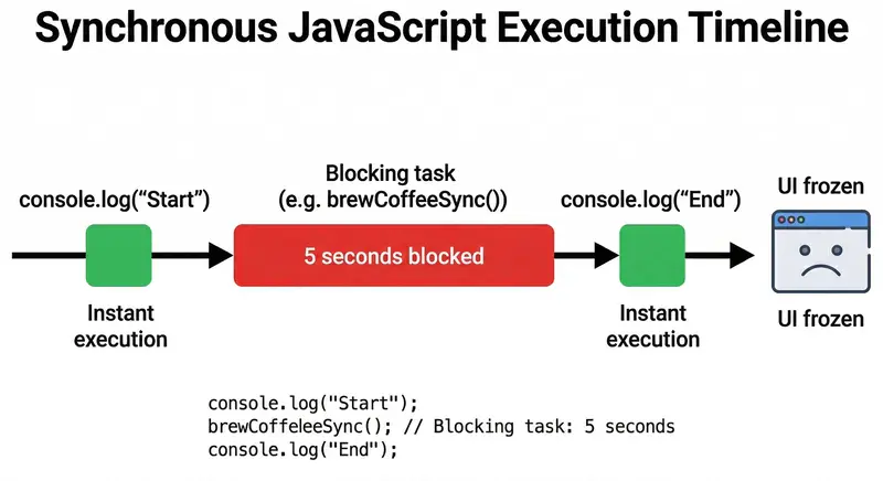
Introduction: The Challenge of Time Series Data in PostgreSQL

Handling large-scale time series data in PostgreSQL, particularly in tables like candle_data, exposes inherent limitations of general-purpose databases when pushed to their limits. The mechanical process of ingesting, storing, and querying time series data in PostgreSQL involves row-based storage and sequential disk I/O, which degrades under high write throughput and complex temporal queries. For instance, as the candle_data table grows, index bloat and disk contention become observable effects, leading to query latency spikes. This is exacerbated by PostgreSQL’s lack of native optimizations for time series workloads, such as columnar compression or vectorized execution, which are critical for reducing storage overhead and accelerating analytical queries.

Performance Bottlenecks in PostgreSQL

The root cause of performance degradation lies in PostgreSQL’s row-oriented storage architecture. When querying time series data, the database must perform full table scans or index lookups, which heat up disk subsystems due to random I/O patterns. For example, a query aggregating data over a 1-year range in candle_data would require scanning millions of rows, causing disk latency to dominate query execution time. While partitioning and indexing strategies (e.g., B-tree indexes on timestamps) can mitigate this, they introduce fragmentation risks and fail to address the fundamental inefficiency of row-based storage for sequential data.

The QuestDB Alternative: Mechanism of Improvement

QuestDB’s columnar storage and vectorized execution engine physically reorganize data to align with time series access patterns. Columns are stored contiguously on disk, enabling sequential reads during range queries, which reduces disk seek time—a critical factor in performance. Additionally, QuestDB’s use of SIMD (Single Instruction, Multiple Data) instructions parallelizes computation at the CPU level, allowing aggregation queries to process entire vectors of data in a single clock cycle. This mechanism directly addresses PostgreSQL’s inefficiencies by minimizing disk I/O and maximizing CPU utilization, resulting in orders-of-magnitude faster query times for time series workloads.

Migration Risks and Edge Cases

Migrating candle_data to QuestDB introduces risks tied to data consistency and operational overhead. During migration, the table’s schema must be translated to QuestDB’s columnar format, which may break compatibility with existing PostgreSQL queries if not handled carefully. For instance, PostgreSQL’s JSONB data type has no direct equivalent in QuestDB, requiring a schema redesign. Partial migration, where candle_data resides in QuestDB while other tables remain in PostgreSQL, further complicates inter-database communication. Without a robust synchronization mechanism (e.g., change data capture), queries spanning both databases risk returning stale or inconsistent data, leading to analytical errors.

Decision Dominance: When to Migrate

Migration to QuestDB is optimal when the following conditions are met: (1) the candle_data table constitutes the majority of storage and query load, (2) query performance degradation in PostgreSQL is directly impacting business metrics (e.g., delayed analytics), and (3) the team can allocate resources for schema migration and QuestDB training. However, if the workload is mixed (e.g., transactional queries dominate), a hybrid architecture may be more effective, with PostgreSQL handling transactional data and QuestDB managing time series. A typical error is underestimating the complexity of inter-database communication, leading to synchronization failures that negate performance gains.

Rule for Choosing Migration:

If time series queries in PostgreSQL exhibit >50% of total query latency and storage costs are escalating linearly with data volume, use QuestDB for candle_data. Otherwise, explore PostgreSQL optimizations (e.g., TimescaleDB) or hybrid architectures to avoid unnecessary operational overhead.

Evaluating QuestDB as a Solution: Features and Benefits

When considering the migration of the candle_data table from PostgreSQL to QuestDB, it’s essential to understand how QuestDB’s architecture addresses the inherent limitations of general-purpose databases for time series workloads. PostgreSQL, with its row-based storage and sequential disk I/O, struggles under high write throughput and complex temporal queries, leading to disk subsystem overheating and index bloat. QuestDB, on the other hand, is purpose-built for time series data, leveraging columnar storage and vectorized execution to minimize disk I/O and maximize CPU utilization.

Here’s how QuestDB’s mechanisms translate into tangible benefits:

• Columnar Storage: Unlike PostgreSQL’s row-oriented design, QuestDB stores columns contiguously on disk. This enables sequential reads, reducing disk seek time and avoiding the random I/O that degrades PostgreSQL’s performance as tables grow. For candle_data, this means faster ingestion and query performance, especially for range-based time series queries.
• Vectorized Execution: QuestDB processes data in vectors using SIMD (Single Instruction, Multiple Data) instructions, allowing it to compute on entire data chunks in a single CPU cycle. This contrasts with PostgreSQL’s scalar execution, which processes one row at a time, leading to underutilized CPU resources and slower query times.
• Time Series Optimizations: QuestDB’s native support for time series data includes timestamp-based partitioning and high-performance append operations, which are critical for handling the high write throughput typical of candle_data. PostgreSQL, without extensions like TimescaleDB, lacks these optimizations, resulting in linear storage cost escalation and query latency spikes.

However, migrating to QuestDB is not without risks. A partial migration of only the candle_data table introduces inter-database communication overhead. For instance, if positions or instruments tables in PostgreSQL need to join with candle_data in QuestDB, the system must handle cross-database queries, which can introduce latency and data consistency risks without proper synchronization mechanisms like change data capture (CDC).

To decide whether QuestDB is the optimal solution, consider the following rule:

Migration Rule: Migrate to QuestDB if candle_data dominates storage and query load, and PostgreSQL query latency exceeds 50% of total application latency, with linear storage cost escalation. Otherwise, optimize PostgreSQL (e.g., with TimescaleDB) or adopt a hybrid architecture to avoid unnecessary overhead.

For example, if candle_data constitutes 80% of the database’s storage and query workload, and PostgreSQL’s query latency for time series calculations is 70% of the total, QuestDB’s columnar storage and vectorized execution could reduce query times by 50-70% while lowering storage costs through efficient compression. However, if candle_data is only 20% of the workload, the migration overhead may outweigh the benefits, and optimizing PostgreSQL with partitioning or indexing might suffice.

In edge cases, such as when candle_data requires real-time analytics with sub-second query response times, QuestDB’s architecture is likely the only viable solution. PostgreSQL, even with optimizations, would struggle to meet such stringent latency requirements due to its row-oriented design and lack of native vectorized execution.

Finally, a common error is underestimating the operational overhead of managing two database systems. Without automation for inter-database communication and data synchronization, the system risks stale data and increased maintenance complexity. A hybrid architecture, while leveraging the strengths of both databases, requires careful planning and resource allocation to avoid these pitfalls.

Migration and Integration Strategies: PostgreSQL to QuestDB

Migrating the candle_data table from PostgreSQL to QuestDB is a strategic move to address the inherent limitations of row-based storage in PostgreSQL for time series data. However, the process requires meticulous planning to avoid data corruption, performance bottlenecks, and synchronization issues. Below is a step-by-step guide grounded in the analytical model and system mechanisms.

1. Data Transfer Methods: Batch vs. Streaming

The choice of data transfer method depends on the data ingestion mechanism in your current PostgreSQL setup. If candle_data is ingested in batches, a batch migration using tools like pg_dump or QuestDB’s COPY command is feasible. For streaming ingestion, a hybrid approach is necessary:

• Batch Migration: Export data from PostgreSQL using COPY TO and import into QuestDB using COPY FROM. This minimizes disk I/O contention in PostgreSQL during export by leveraging sequential reads from disk.
• Streaming Migration: Use a change data capture (CDC) tool like Debezium to replicate incremental changes. This avoids data staleness but introduces latency due to inter-database communication overhead.

Rule: Use batch migration if candle_data is static or infrequently updated. Opt for streaming if real-time data consistency is critical.

2. Schema Adjustments: Mapping PostgreSQL to QuestDB

QuestDB’s columnar storage requires schema adjustments to maximize performance. Key considerations include:

• Timestamp Column: Ensure the timestamp column is explicitly defined as TIMESTAMP in QuestDB to enable vectorized execution and sequential disk reads.
• Data Types: Map PostgreSQL’s JSONB to QuestDB’s STRING or SYMBOL, but beware of query performance degradation due to lack of native JSON support in QuestDB.
• Partitioning: Leverage QuestDB’s timestamp-based partitioning to reduce disk seek time and improve query performance for time-range queries.

Rule: Prioritize timestamp alignment and partitioning to exploit QuestDB’s columnar storage. Avoid complex data types like JSONB unless absolutely necessary.

3. Minimizing Downtime: Parallel Operation and Cutover Strategy

To minimize downtime, adopt a parallel operation strategy where both databases serve queries during migration. This requires:

• Read/Write Splitting: Route writes to both PostgreSQL and QuestDB during migration to maintain data consistency. Use a synchronization mechanism like CDC to replicate changes.
• Cutover Plan: Once migration is complete, switch read traffic to QuestDB. Monitor for query latency spikes due to unoptimized schema or indexing.

Rule: If downtime tolerance is low, implement parallel operation. Otherwise, schedule migration during off-peak hours and perform a direct cutover.

4. Inter-Database Communication: Synchronization Mechanisms

Partial migration introduces inter-database communication overhead, which can degrade performance. To mitigate this:

• CDC with Debezium: Replicate changes from PostgreSQL to QuestDB in near real-time. This minimizes data staleness but adds network latency.
• ETL Pipelines: Use batch ETL processes for non-critical data. This reduces network congestion but introduces data lag.

Rule: Use CDC for real-time synchronization if candle_data is frequently queried. Otherwise, opt for batch ETL to reduce operational overhead.

5. Edge-Case Analysis: Hybrid Architecture vs. Full Migration

A hybrid architecture (PostgreSQL for transactional data, QuestDB for time series) may seem appealing but carries risks:

• Performance Trade-offs: Cross-database queries can introduce latency spikes due to network hops and lack of join optimization between databases.
• Operational Complexity: Managing two databases increases maintenance overhead and requires robust automation for synchronization.

Rule: Opt for a hybrid architecture only if candle_data is decoupled from other tables. Otherwise, fully migrate to QuestDB to avoid inter-database dependencies.

6. Benchmarking and Validation

Before committing to QuestDB, conduct performance benchmarks to quantify improvements. Key metrics include:

• Query Latency: Compare PostgreSQL and QuestDB for time-range queries. QuestDB should show 50-70% reduction due to vectorized execution.
• Ingestion Throughput: Measure write performance under high load. QuestDB’s append-optimized storage should outperform PostgreSQL’s row-based inserts.

Rule: Migrate only if benchmarks confirm significant performance gains. Otherwise, optimize PostgreSQL with TimescaleDB or partitioning.

Conclusion: Decision Dominance

Migrating candle_data to QuestDB is optimal if:

• Time series queries dominate latency and storage costs in PostgreSQL.
• Benchmarks show 50%+ improvement in query performance with QuestDB.
• Resources are available for schema migration and team training.

Otherwise, optimize PostgreSQL with TimescaleDB or adopt a hybrid architecture. Avoid partial migration without robust synchronization mechanisms, as it risks data inconsistency and operational complexity.

Communication and Query Optimization Between Databases

Migrating the candle_data table from PostgreSQL to QuestDB introduces a hybrid database environment, where seamless communication and query optimization become critical. The challenge lies in balancing the strengths of both systems while mitigating the risks of inter-database dependencies. Here’s a deep dive into the strategies, mechanisms, and trade-offs involved.

1. Data Synchronization Mechanisms

Partial migration of candle_data creates a risk of data inconsistency due to the temporal mismatch between PostgreSQL’s row-based updates and QuestDB’s append-optimized writes. The causal chain is as follows:

• Impact: Stale data in one database leads to incorrect calculations or analytics.
• Internal Process: Without real-time synchronization, writes to PostgreSQL are not immediately reflected in QuestDB, causing a lag.
• Observable Effect: Queries spanning both databases return inconsistent results, degrading trust in the system.

To address this, Change Data Capture (CDC) with tools like Debezium is optimal. CDC captures row-level changes in PostgreSQL and streams them to QuestDB, ensuring near real-time consistency. However, this introduces network latency due to inter-database communication. For less critical data, ETL pipelines can batch updates, reducing overhead but increasing lag.

Rule: Use CDC for frequently queried data; ETL for reduced operational overhead.

2. Query Routing and Optimization

Cross-database queries are inherently slower due to the network hop between PostgreSQL and QuestDB. The mechanism is:

• Impact: Latency spikes degrade application performance.
• Internal Process: Data must be fetched from both databases, serialized, and combined in the application layer.
• Observable Effect: Slow response times for queries involving candle_data and other PostgreSQL tables.

To optimize, denormalize data where possible, storing pre-aggregated results in QuestDB to reduce joins. Alternatively, use federated queries with a query router (e.g., Apache Calcite) to intelligently route queries to the appropriate database. However, federated queries add complexity and require careful tuning.

Rule: Denormalize if possible; use federated queries only if the schema allows decoupling.

3. Hybrid Architecture vs. Full Migration

A hybrid architecture retains PostgreSQL for transactional data while offloading time series data to QuestDB. The trade-off is:

• Benefit: Leverages PostgreSQL’s strengths for user management and transactional consistency.
• Risk: Increased operational overhead due to dual database management and potential latency spikes.

Full migration eliminates inter-database dependencies but requires rewriting queries and retraining the team. The decision hinges on the coupling of data between candle_data and other tables.

Rule: Hybrid only if data is decoupled; otherwise, fully migrate to avoid complexity.

4. Benchmarking and Validation

Before committing to migration, benchmark PostgreSQL and QuestDB with representative workloads. The key metrics are:

• Query Latency: Expect 50-70% reduction in QuestDB due to vectorized execution.
• Ingestion Throughput: QuestDB’s append-optimized storage outperforms PostgreSQL’s row-based inserts.

If benchmarks do not show significant gains, consider optimizing PostgreSQL with TimescaleDB instead. The mechanism is:

• Impact: Suboptimal performance despite migration.
• Internal Process: QuestDB’s optimizations are not fully utilized due to workload mismatch.
• Observable Effect: Wasted resources and no tangible improvement.

Rule: Migrate if benchmarks show significant gains; otherwise, optimize PostgreSQL.

5. Edge Cases and Failure Modes

Consider edge cases where the chosen solution may fail:

• Real-time Analytics: QuestDB is the only viable solution for sub-second query response times due to its architecture.
• Schema Incompatibility: PostgreSQL’s JSONB has no direct QuestDB equivalent, requiring schema redesign.
• Rollback Challenges: Reverting to PostgreSQL post-migration is costly due to data format differences and query rewrites.

Rule: Avoid partial migration without robust synchronization; plan for rollback if QuestDB does not meet expectations.

Conclusion

Migrating candle_data to QuestDB offers significant performance gains but requires careful planning to manage inter-database communication and data consistency. The optimal strategy depends on the workload, data coupling, and resource constraints. For decoupled data, a hybrid architecture may suffice; otherwise, full migration is recommended. Always benchmark and validate before committing to ensure the expected benefits materialize.

There’s a moment every software engineer knows.

You’re explaining a new feature to a teammate. The schema is in your head. You need something visual, fast, right now. You open a browser tab, type dbdiagram.io, and in three minutes you have a diagram you can paste into Slack.

The meeting happens. Everyone nods. The diagram link dies in the chat history. The actual schema lives in your database, unrelated to what you drew.

That’s not a failure of discipline. That’s the ceiling of the tool.

This article is for engineers who have hit that ceiling and are wondering what comes next.

The Honest Summary

dbdiagram.io is a fast, focused ERD tool built for quick sketching. Fast, free, browser-based, zero friction. If you need a diagram for a meeting and you’ll never look at it again, nothing beats it.

Schemity is what you use when the diagram needs to outlive the meeting. When your ERD is part of your codebase, not a link in Slack. When you want to go from sketch to production schema without switching tools.

If that distinction doesn’t matter to you yet, use dbdiagram.io. It’s genuinely excellent at what it does.

If it does matter, read on.

Side-by-Side

Where dbdiagram.io Wins

Let’s be honest about this. dbdiagram.io does several things better than almost any alternative.

Speed from zero. No download. No account required. Open browser, start typing, diagram appears in real time. For the specific use case of “I need an ERD right now,” nothing is faster.

DBML syntax. If you think in code, DBML is elegant. Define a table in four lines. Copy it from your ORM model. The keyboard never leaves the home row. For engineers who find drag-and-drop slower than typing, this is genuinely the right interface.

Sharing is trivial. One link. Anyone can view it. No account needed for viewers. For sharing with non-technical stakeholders or across teams, the link-based sharing model is hard to beat.

Free. For individual use up to 10 diagrams, you pay nothing. For a lot of engineers, that’s enough.

Where dbdiagram.io Hits Its Ceiling

The diagram is not your schema. It’s a picture of your schema.

This is the fundamental problem. dbdiagram.io creates a visualization. It doesn’t connect to your database. It doesn’t track changes. It doesn’t generate migrations. When your schema evolves (and it always does), your diagram falls behind. Within weeks, the link you shared is a historical artifact, not a current document.

Your data lives on their servers, not yours.

Every diagram you create in dbdiagram.io is stored on Holistics’ infrastructure. If they shut down, your diagrams disappear. If your company requires data locality (SOC 2, ISO 27001, regulated industries), a browser tool storing your schema on a third-party server is a compliance question you’d rather not answer.

The free tier is a public diagram trap.

The free tier gives you 10 diagrams, all public, all visible to anyone with the link, with no private option. The moment you need diagram number 11, or your first private diagram, the pricing jumps to $9/month. For most engineers working on real projects, “public diagrams only” is a non-starter from day one. Your schema is not a public document.

No offline.

Working on a flight. Behind a corporate firewall. On a client site with restricted internet. dbdiagram.io simply doesn’t work. For a tool that’s supposed to help you think through your architecture, internet dependency is a real constraint.

DBML has a learning curve for non-coders.

If you’re the senior engineer who thinks in SQL, DBML feels natural. If you’re onboarding a junior, or collaborating with a data analyst who doesn’t write SQL daily, the code-first interface creates friction. The visual feedback is good, but the input method is a barrier.

The Three Failure Modes Schemity Was Built to Solve

Schemity wasn’t built to compete with dbdiagram.io on its own terms. It was built to solve three specific failure modes that exist across the entire ERD tool market.

Failure Mode 1: The tool defeats you before you start

Visual Paradigm is a serious modeling tool. It does have a Community edition that is free. But finding it is its own obstacle. The download page is cluttered with editions, pricing tiers, and license options that make it genuinely unclear which version to download. Engineers who just want to start modeling end up reading licensing FAQs instead of drawing tables.

Once you do find the right download, the installer takes over. JVM dependency, license wizard, 200+ MB download. Motivated engineers have abandoned it before creating a single entity. The tool defeated them before they opened it.

Schemity is 9 MB. It starts in seconds. There is no IT ticket, no JRE installation, no license wizard, no edition confusion. One download, one version, running immediately. The activation energy is low enough that you open it before the meeting, not after.

Failure Mode 2: Fast sketching and serious design are mutually exclusive

The market has forced a false choice: either use a basic tool that’s fast (dbdiagram.io) or use an enterprise tool that’s serious (Visual Paradigm, erwin). There is almost nothing in between.

Schemity is drag-and-drop fast. Keyboard shortcuts make it faster still once you’re comfortable. But the same tool that handles a five-minute sketch also handles a production schema with 100+ tables, composite unique constraints, check constraints, indexes, and SSH-connected live database sync. It can also generate SQL migrations directly from your ERD, useful for personal projects and fast POCs where you don’t need a full migration framework in the way. For production team workflows, your existing migration tooling stays in charge. Schemity sits alongside it, not in front of it.

You don’t graduate to another tool. You just use more of the same tool.

Failure Mode 3: Trial expiry holds your work hostage

This is the fear nobody talks about in ERD tool marketing. You spend two hours in a trial. The trial expires. Your diagrams are either gone or locked behind a paywall. And if you were on dbdiagram.io’s free tier the whole time, your schema was public to anyone with the link. Serious, sensitive work sitting on a public URL without you realizing it.

Schemity’s answer to this is architectural, not a policy. Your ERDs are plain JSON files in ~/schemity/ on your own machine. When the trial expires, Schemity stops receiving updates. You get a single friendly reminder when you open the app, once per session, not a popup that blocks your work or repeats every five minutes. Everything else works exactly as before. Your files are yours. They always were.

If Schemity shuts down as a business tomorrow, your diagrams open perfectly on Monday.

The Git Workflow Nobody Else Has

This is the feature that changes how a team works with database design.

In dbdiagram.io, your ERD lives at a URL. You share the link. When the schema changes, someone updates the diagram manually, if they remember. The diagram and the codebase drift apart over time. Within months, the link you shared in Slack is a historical artifact, not a current document.

Schemity takes a fundamentally different approach, one borrowed from how mature engineering teams already handle infrastructure.

Nobody commits Terraform files inside an application service repo. Infrastructure is a shared concern, it spans services, it has its own change cadence, it deserves its own review. So it lives in its own repo.

Your database schema deserves the same treatment.

The pattern Schemity enables is an ERD repo: a single, dedicated repository that holds the ERDs for every service in your company.

company-erd-repo/
  ├── payment-service/
  ├── user-service/
  ├── notification-service/
  └── legacy-crm/

Each folder is a Schemity workspace containing plain JSON files. The entire repo lives as ~/schemity/ on every engineer’s machine. Schemity opens it as a central hub.

Schemity does not stand in your workflow. It does not replace your migration tool. Your schema changes still flow through whatever your team already uses: Django, Rails, Flyway, Atlas, anything. Schemity sits alongside that workflow, not in front of it.

Here is what it looks like in practice:

For the engineer making the change: Clone company-erd-repo once into ~/schemity/. Run your migration as normal. Once it is applied to your local database, open Schemity, connect to it, and let it reflect the current state. Arrange the entities, update the relationships, add legends to give the diagram business meaning. Commit the updated JSON and open a PR against the ERD repo.

For the engineer reviewing the change: Pull the branch. Open Schemity. The diff is right there, a JSON file change that maps directly to a visual diagram. No migration file archaeology. No mental reconstruction of what the schema looked like before.

For the architect reviewing multiple services: One repo. One clone. Every service’s schema in one place. No hopping between repos hoping someone committed a diagram.

For the new engineer onboarding:

git clone [email protected]:company/erd-repo.git ~/schemity

One command. Every service. Every relationship. Every constraint. The full picture of the company’s data model, version-controlled and up to date.

What this unlocks that dbdiagram.io never can:

Schema changes get reviewed like code. When a schema change requires a PR against the ERD repo, the change gets reviewed before it is applied, not after. The history of every schema decision lives in Git: who changed it, when, and why.

The database is always the source of truth. Real teams miss steps. An engineer ships a migration in a busy sprint and forgets to update the ERD. It happens. With dbdiagram.io, that diagram is now wrong and nobody knows it. With Schemity, the next time anyone opens that ERD and connects to the database, Schemity reflects the current state automatically. The new tables are there. The new relationships are there. The new columns are there. The only thing missing is the visual arrangement: where the entities sit on the canvas and how the lines are routed. Drag a few boxes, tidy the lines, commit. No data lost. Nothing out of date. The diagram catches up in minutes, not sprint cycles.

This is separation of concerns applied to the full engineering stack. Source code in service repos. Infrastructure in the infra repo. Schema in the ERD repo.

It is not a feature dbdiagram.io can add. It would require rethinking what an ERD tool is for.

Pricing: One-Time vs. Monthly

dbdiagram.io: $9/month ($108/year) once you exceed the free tier.

Schemity: $129 one-time with $69/year renewal for updates (optional, the tool works forever without renewing).

At 14 months, Schemity costs the same as dbdiagram.io’s subscription. Every month after that, Schemity is free. If you use it for three years (and engineers tend to stick with tools that work), Schemity costs $129 + $138 = $267 total. dbdiagram.io costs $324 for the same period, and you still don’t own it.

The more important pricing difference is philosophical. Schemity’s one-time model is a statement: the tool is valuable enough that you’ll keep using it without being forced to. You don’t stay because canceling is painful. You stay because the tool earns it.

Who Should Use dbdiagram.io

• You need a diagram in the next five minutes for a meeting
• You’ll never look at this diagram again after today
• You’re communicating a schema idea, not building one
• You think in DBML and the code-first interface is faster for you
• The diagram doesn’t need to live anywhere except a Slack link

dbdiagram.io is excellent for this use case. Use it without guilt.

Who Should Use Schemity

• You need the diagram to still be accurate next month
• Your ERD belongs in your repository, not in someone else’s cloud
• You work offline, behind a VPN, or in a restricted environment
• You’re graduating from a basic tool without wanting a tool that feels like an enterprise installation ceremony
• You want to generate migrations directly from your design for a personal project or fast POC, without a full migration framework in the way
• You’re a senior engineer recommending a tool to a junior who shouldn’t be defeated by the installer

The Bottom Line

dbdiagram.io is a sketch pad. It’s a very good sketch pad.

Schemity is a design tool that happens to be as fast as a sketch pad.

The question is not which tool is better in absolute terms. The question is whether your ERD is a communication artifact that lives in a meeting, or a design artifact that lives in your codebase.

If it’s the latter, Schemity was built for you.

If Schemity sounds like the right fit, you can grab it at schemity.com, 9 MB, 2-week full trial, no account required.

A coding agent just suggested adding a package to your project. You’ve never heard of it. How do you decide whether to trust it?

Most developers either accept the suggestion blindly or spend fifteen minutes checking GitHub stars, last commit date, the npm advisory database, and whatever license file happens to exist. Agents can’t do either — they need a structured signal, fast.

The data exists. It’s just scattered.

The information you need to evaluate a dependency already exists across public APIs. OSV.dev maintains a comprehensive vulnerability database covering CVEs and GitHub Security Advisories across npm, PyPI, Go, Rust, and more. Google’s deps.dev aggregates dependency graphs, license metadata, and OpenSSF Scorecard results — the 18-check security health assessment that most developers have never heard of despite it covering over a million projects. The npm and PyPI registries themselves tell you when a package was last published, whether it’s deprecated, and how many maintainers it has.

The problem isn’t data availability. It’s that these are five or six separate HTTP calls with different request formats, different response schemas, and different failure modes. An agent checking one dependency has to call OSV.dev with a POST body specifying ecosystem and version, then hit deps.dev’s REST API to get the linked GitHub project, then make another call to deps.dev for the OpenSSF Scorecard, then query the registry for freshness signals. Then it has to synthesize all of that into a decision. Multiply that by forty dependencies in a lockfile and you’ve built an integration project, not a quick check.

What we built

package-security-audit aggregates all of the above into a single API call. You pass a package name and optionally a version and ecosystem. It calls OSV.dev, deps.dev, and the relevant registry in parallel, normalizes everything, and returns a 0–100 risk score with the evidence behind it.

curl -X POST https://api.strale.io/v1/do 
  -H "Authorization: Bearer $STRALE_API_KEY" 
  -H "Content-Type: application/json" 
  -d '{
    "capability_slug": "package-security-audit",
    "inputs": { "name": "express", "version": "4.18.2" }
  }'

Here’s what comes back (trimmed to the output fields):

{
  "output": {
    "name": "express",
    "version": "4.18.2",
    "ecosystem": "npm",
    "risk_score": 94,
    "risk_level": "low",
    "vulnerabilities": {
      "total": 2,
      "critical": 0,
      "high": 0,
      "medium": 0,
      "low": 2,
      "details": [
        {
          "id": "GHSA-qw6h-vgh9-j6wx",
          "severity": "low",
          "summary": "express vulnerable to XSS via response.redirect()",
          "fixed_in": "4.20.0"
        },
        {
          "id": "GHSA-rv95-896h-c2vc",
          "severity": "moderate",
          "summary": "Express.js Open Redirect in malformed URLs",
          "fixed_in": "4.19.2"
        }
      ]
    },
    "license": {
      "spdx": "MIT",
      "is_osi_approved": true,
      "is_copyleft": false
    },
    "freshness": {
      "latest_version": "5.2.1",
      "is_latest": false,
      "is_deprecated": false,
      "days_since_last_release": 121
    },
    "maintainers": 5,
    "dependency_count": 0
  },
  "provenance": {
    "source": "osv.dev + deps.dev + registry",
    "fetched_at": "2026-04-02T10:30:33.440Z"
  }
}

Express 4.18.2 scores 94/100 — low risk. Two low-severity vulnerabilities, both with known fix versions. MIT license, five maintainers, not deprecated. The only flag: it’s not the latest version (5.2.1 is out). An agent can read that response and make a decision in milliseconds. The whole call took 486ms.

The second capability, license-compatibility-check, handles a different question: given a set of licenses across your dependency tree, are they all compatible with your use case?

curl -X POST https://api.strale.io/v1/do 
  -H "Authorization: Bearer $STRALE_API_KEY" 
  -H "Content-Type: application/json" 
  -d '{
    "capability_slug": "license-compatibility-check",
    "inputs": {
      "licenses": ["MIT", "Apache-2.0", "GPL-3.0-only"],
      "use_case": "commercial"
    }
  }'

{
  "output": {
    "compatible": false,
    "use_case": "commercial",
    "license_count": 3,
    "licenses_analyzed": [
      { "input": "MIT", "type": "permissive", "compatible_with_use_case": true },
      { "input": "Apache-2.0", "type": "permissive", "compatible_with_use_case": true },
      { "input": "GPL-3.0-only", "type": "strong_copyleft", "compatible_with_use_case": false }
    ],
    "conflicts": [
      {
        "licenses": ["GPL-3.0-only"],
        "reason": "GPL-3.0-only is strong copyleft — requires distributing your source code under the same license. Incompatible with proprietary commercial distribution.",
        "severity": "error"
      }
    ],
    "summary": "1 compatibility conflict(s) found for commercial use. Strong copyleft licenses detected."
  }
}

It covers 30+ SPDX licenses and knows the specific compatibility rules that trip people up — GPL-2.0 and GPL-3.0 are mutually incompatible unless “or-later” is used, Apache-2.0 conflicts with GPL-2.0-only, and AGPL in any dependency makes your entire SaaS project AGPL-bound. Purely algorithmic, 8ms response time.

The dependency-risk-check solution chains both: security audit plus license compatibility in a single call for €0.25.

How it works under the hood

The security audit makes four parallel requests. OSV.dev gets queried with the specific package version and ecosystem to find known vulnerabilities. deps.dev provides the license, dependency count, and a link to the source repository. If that repository is on GitHub, a second deps.dev call fetches the OpenSSF Scorecard — an automated assessment of 18 security practices including branch protection, code review, dependency update tooling, and fuzzing coverage. The registry API supplies freshness and deprecation data.

Penalties are applied to a starting score of 100: critical CVEs cost 25 points each, deprecated packages lose 20, packages not updated in over two years lose 20, and missing licenses lose 15. The floor is zero. If any upstream source is temporarily unavailable, the remaining sources still produce a partial score rather than failing the entire call.

Every response includes provenance metadata — which sources were queried and when — so the agent or human reviewing the decision can trace where the data came from.

For agent builders

The practical use case is making npm install or pip install a decision an agent can make autonomously. With Strale’s MCP server, a coding agent can check any package before adding it — no configuration, no API keys to manage beyond the Strale key.

npx strale-mcp

Any MCP-compatible client (Claude Code, Cursor, Windsurf, or anything else speaking the protocol) can call package-security-audit directly. The agent gets back structured JSON it can reason over: a numeric risk score, specific vulnerabilities with fix versions, and a clear compatible/incompatible verdict on licensing. That’s enough to make an autonomous yes/no decision, or to surface a warning to the developer when the score is marginal.

package-security-audit costs €0.15 per call. license-compatibility-check costs €0.05. That’s cheap enough to check every dependency in a typical lockfile for under €10.

Both capabilities are live now. The API docs have the full input/output schemas, or you can browse the capability catalog to see them alongside the 270+ other capabilities available. The source is at github.com/strale-io.