MPT DEX Performance Test Report

Introduction

The MPTVersion2 amendment (XLS-82) extends Multi-Purpose Token (MPT) support to the XRP Ledger’s Decentralized Exchange (DEX), enabling MPT assets to participate natively in Automated Market Maker (AMM) pools, order book offers, cross-currency payments, and check-based transfers. This builds directly on the XLS-33 MPT foundation and the existing XRPL DEX infrastructure (XLS-30).

Rather than introducing new on-ledger objects or a separate trading engine, MPTVersion2 extends existing transaction types — AMMCreate, AMMDeposit, AMMWithdraw, AMMClawback, AMMDelete, CheckCreate, CheckCash, OfferCreate, and Payment — to treat MPT as a first-class asset alongside XRP and IOUs. MPT amounts are identified by mpt_issuance_id in transaction JSON in place of the currency/issuer fields used by IOUs.

This report summarizes a comprehensive performance evaluation of the MPTVersion2 amendment under high-load conditions. Tests were executed in RippleX’s private performance network to quantify throughput, consensus latency, CPU/memory utilization, and regression impact relative to the 3.1.2 release baseline.

The results demonstrate that MPT DEX integration is performant and stable, with no material regression against baseline IOU-based DEX operations, and that the amendment can be safely activated without compromising the 5-second consensus target.

Executive Summary

The MPTVersion2 amendment introduces no measurable performance regression against the 3.1.2 production release. Under identical conditions, the mpt_dex build matched baseline throughput within 0.4%. Pure MPT path payments outperformed the IOU baseline by 14.2%, while the most complex mixed MPT-IOU paths came within 1.7% of baseline. DEX transaction capacity with MPT token pairs exceeded IOU equivalents by over 36%. All scenarios maintained consensus latency below the 5-second target across both 1-hour and 5-hour endurance runs, with stable CPU and memory utilization throughout. The amendment is safe to activate without compromising MainNet SLOs.

Testing Objectives

The primary objective of this testing was to assess the performance impact of enabling MPT assets in DEX and payment flows, and to validate that no regressions are introduced relative to the 3.1.2 production release. Specifically, we aimed to:

  • Establish a clean performance baseline comparing the mpt_dex build against the 3.1.2 release under identical load and database conditions.
  • Validate that the mpt_dex build performs equivalently when run against both the baseline performance database and the MPT DEX-enriched database, confirming that MPT ledger object population does not degrade existing transaction performance.
  • Measure the throughput, consensus latency, and resource utilization of MPT-enabled path payments across multiple path complexity tiers.
  • Compare MPT path payment performance across three middle path configurations — pure IOU-IOU (baseline), pure MPT-MPT, and alternating MPT-IOU — at increasing path complexity tiers.
  • Stress test rippled’s DEX transaction processing under a load distribution mirroring the most frequent MainNet operations (AMMCreate, AMMDeposit, OfferCreate) with MPT/MPT token pairs, validating no regression against the IOU-only baseline.
  • Ensure that the network consistently maintains a 5-second consensus latency threshold under all test scenarios.

Testing Methodology

Capacity Planning

The 5-second consensus latency limit serves as the benchmark for network capacity across all scenarios. This threshold ensures the network remains in optimal condition while processing a mix of MPT-enabled DEX, AMM, and payment transactions alongside standard payment flows. Instances where the network surpassed this limit are referred to as “overvalidation” in the results below.

Test Environment

Testing was conducted in a private XRPL environment with 9 nodes, mirroring Ripple’s MainNet hardware specifications.

Network Setup

  • 5 nodes function as validator nodes
  • 4 nodes serve as client P2P nodes, interfacing with load generators
  • All nodes are hosted on AWS EC2 z1d.2xlarge instances: 8 CPU cores, 64 GB RAM, 300 GB NVMe SSD
  • All nodes operate within the same AWS region, interconnected via a shared LAN
  • Between 1 and 4 load servers transmit transactions to the 4 P2P nodes

Account Setup

A total of 250,000 synthetic accounts were established, built atop a public ledger synchronized from MainNet. 15 accounts were designated as MPT token issuers, distributing MPT balances to the remaining MPT participant accounts.

rippled Configuration

The rippled configuration was sourced from a Ripple MainNet validator, with modifications made only as required for the test environment.

Test Data Setup

Multi-Purpose Token Initialization

To support MPT-backed DEX testing, the environment was pre-initialized with MPT objects following the XLS-33 and XLS-82 specifications.

Three token chains were constructed to support the full range of path payment scenarios:

IOU1 → IOU2 → IOU3 → IOU4 → IOU5 → IOU6 → IOU7 → IOU8

MPT1 → MPT2 → MPT3 → MPT4 → MPT5 → MPT6 → MPT7 → MPT8

MPT1 → IOU1 → MPT2 → IOU2 → MPT3 → IOU3 → MPT4 → IOU4

The pure IOU chain serves as the baseline control. The pure MPT chain exercises MPT-only pathfinding. The alternating MPT-IOU chain represents the most complex cross-type routing scenario, requiring the pathfinding engine to resolve offer crossings between MPTokenIssuance and trust line objects at every hop.

Database creation followed this sequence:

  1. Issuer accounts created MPT issuances via MPTokenIssuanceCreate, with lsfMPTCanTrade and lsfMPTCanTransfer flags set to enable DEX participation.
  2. All holder accounts were authorized via MPTokenAuthorize.
  3. Token issuers funded root accounts via Payment.
  4. All four load servers distributed MPT balances to the full holder population.
  5. AMM pools and order book offers were pre-created to seed liquidity across the full asset graph.

Load Modeling

Scenario 1 — Baseline: Build Regression (mpt_dex vs. 3.1.2 Release)

Objective: Confirm that the mpt_dex build introduces no performance regression against the current 3.1.2 production release under identical baseline conditions.

Two sub-comparisons were performed:

1a. Baseline DB — 5-Hour Build Comparison

Both builds executed against the standard 250K account baseline performance database (no MPT objects). This isolates code-level regressions introduced by the MPTVersion2 amendment independent of ledger state changes.

  • Load: Standard IOU mixed payment load (XRP-XRP, IOU Direct, AMM/LOB 1path1step, 3path3step, 6path8step)
  • No MPT transactions included
Scenario Ledger throughput per second Mean Ledger Publishing Latency (s) P95 Ledger Publishing Latency (s) Average Response Time (ms) Over Validation CPU Utilization (%) Memory Usage (GB / Total)
3.1.2 Release 160.84 4.03 4.72 9.25 30 out of 4476 12.4 17.6/64 GB
mpt_dex build 160.29 4.07 4.80 9.59 32 out of 4438 12.5 17.9/64 GB

1b. mpt_dex Build — 5-Hour DB Comparison (Baseline DB vs. MPT DEX DB)

The mpt_dex build was tested against both the baseline database and the MPT DEX-enriched database (populated with MPT issuances, MPToken objects, new AMM pools, and offers) under the same standard mixed payment load. This validates that MPT ledger object population does not degrade performance for non-MPT transactions.

Scenario Ledger throughput per second Mean Ledger Publishing Latency (s) P95 Ledger Publishing Latency (s) Response Time (ms) Over Validation CPU Utilization (%) Memory Usage (GB / Total)
Baseline DB 159.45 4.06 4.78 9.75 31 out of 4451 11.7 18.9/64 GB
MPT DEX DB 159.20 4.08 4.83 10.05 44 out of 4423 12.3 19.8/64 GB

Scenario 2 — MPT DEX Path Payments

Objective: Measure throughput, latency, and resource impact of MPT-enabled cross-currency path payments at increasing path complexity, compared against an IOU-only baseline.

All three configurations below were tested under a mixed load combining all three path complexity tiers simultaneously:

Path Complexity Description
1 path / 1 step Direct single-hop payment
3 paths / 3 steps Moderate path fan-out
6 paths / 8 steps Worst-case routing complexity

2a. IOU-IOU Middle Path — Baseline (Control)

Pure IOU-to-IOU payments routed through IOU intermediate hops. No MPT involvement. Used as the regression control for all path payment comparisons.

Path structure:

IOU1 → IOU2 → IOU3 → ... → IOU8
Scenario Ledger throughput per second Mean Ledger Publishing Latency (s) P95 Ledger Publishing Latency (s) Response Time (ms) Over Validation CPU Utilization (%) Memory Usage (GB / Total)
IOU-IOU Middle Path 142.89 3.92 4.59 9.42 4 out of 932 11.4 16.8/64 GB

2b. MPT-MPT Middle Path — Pure MPT

MPT-to-MPT payments routed exclusively through MPT intermediate hops. This exercises MPTokenIssuance and MPToken state lookups at every step of the payment path, with no trust line traversal involved.

Path structure:

MPT1 → MPT2 → MPT3 → ... → MPT8
Scenario Ledger throughput per second Mean Ledger Publishing Latency (s) P95 Ledger Publishing Latency (s) Response Time (ms) Over Validation CPU Utilization (%) Memory Usage (GB / Total)
MPT-MPT Middle Path 163.24 3.99 4.59 11.79 3 out of 918 11.7 16.9/64 GB

2c. MPT-IOU Alternating Middle Path

MPT-to-MPT source/destination payments routed through an alternating sequence of MPT and IOU intermediate hops. This is the most complex path payment configuration, requiring the pathfinding engine to resolve cross-type offer crossings at every step, alternating between MPTokenIssuance and trust line state lookups.

Path structure:

MPT1 → IOU1 → MPT2 → IOU2 → MPT3 → ...
Scenario Ledger throughput per second Mean Ledger Publishing Latency (s) P95 Ledger Publishing Latency (s) Response Time (ms) Over Validation CPU Utilization (%) Memory Usage (GB / Total)
MPT-IOU Middle Path 140.46 3.98 4.73 12.05 3 out of 921 11.8 17.2/64 GB

2d. Endurance Testing across three scenarios

To validate stability under sustained load, all three path payment configurations were run continuously for 5 hours. The objective was to confirm consistent throughput, detect any anomalous degradation over time, and observe CPU and memory behavior beyond the initial ramp-up period.

Scenario Ledger throughput per second Mean Ledger Publishing Latency (s) P95 Ledger Publishing Latency (s) Response Time (ms) Over Validation CPU Utilization (%) Memory Usage (GB / Total)
IOU-IOU Middle Path 142.56 4.03 4.75 9.72 34 out of 4476 12.3 17.6/64GB
MPT-MPT Middle Path 163.15 4.04 4.77 11.67 24 out of 4475 12.2 17.7/64GB
MPT-IOU Middle Path 140.35 4.09 4.84 12.93 24 out of 4416 12.4 18.9/64GB

Endurance Testing System Utilization Graph

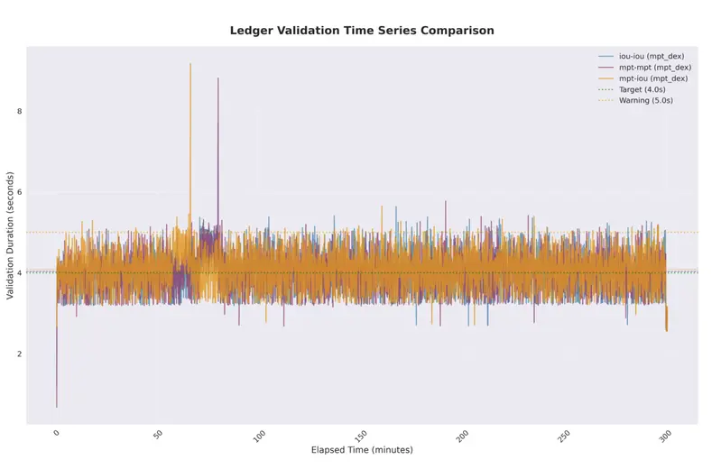
Ledger Validation Time

Ledger validation time increases with scenario complexity, progressing from IOU-IOU through MPT-MPT to MPT-IOU. All validation times remain below the 5-second target threshold.

Memory Usage Analysis

This chart displays normal memory behavior, with usage stabilizing after an initial ramp-up and then holding steady.

IOU-IOU Middle Path MPT-MPT Middle Path MPT-IOU Middle Path

CPU Usage Analysis

This chart shows stable and low CPU utilization for validator nodes. The spikes are result from the online delete being triggered during the tests.

IOU-IOU Middle Path MPT-MPT Middle Path MPT-IOU Middle Path

Scenario 3 — OfferCreate & AMM Capacity

Objective: Assess the performance impact of MPT DEX support on high-frequency DEX transaction types. The load distribution is modeled on observed MainNet DEX traffic, where OfferCreate, AMMDeposit, and AMMCreate are among the most common operations. By comparing IOU-only against MPT/MPT token pair configurations under the same transaction mix, this scenario quantifies how MPT asset support affects DEX throughput and consensus stability.

The load mix mostly reflects the observed MainNet DEX distribution: 80% OfferCreate, 18% AMMDeposit, and 2% AMMCreate.

3a. 1-Hour Capacity Run — IOU/IOU vs. MPT/MPT

Both token pair configurations were tested under the same load mix. IOU/IOU serves as the regression control; MPT/MPT exercises all MPT-specific flag and authorization checks on both legs of every OfferCreate, AMMDeposit, and AMMCreate transaction.

Scenario Ledger throughput per second Mean Ledger Publishing Latency (s) P95 Ledger Publishing Latency (s) Response Time (ms) Over Validation CPU Utilization (%) Memory Usage (GB / Total)
IOU-IOU 207.43 3.89 4.18 8.33 0 out of 940 12.1 16.3/64GB
MPT-MPT 282.57 3.86 4.17 7.58 0 out of 948 13.1 16.9/64GB

3b. 5-Hour Endurance Testing

Extended longevity runs were conducted to monitor system stability, CPU utilization, and memory growth trends under sustained DEX load with MPT token pairs.

Scenario Ledger throughput per second Mean Ledger Publishing Latency (s) P95 Ledger Publishing Latency (s) Response Time (ms) Over Validation CPU Utilization (%) Memory Usage (GB / Total)
IOU-IOU 206.85 4.34 4.18 8.91 12 out of 4589 13.3 17.1/64GB
MPT-MPT 281.11 4.27 4.17 8.15 16 out of 4634 14.3 18.2/64GB

Conclusion

The performance evaluation of the MPTVersion2 amendment (XLS-82) demonstrates no material regression against the 3.1.2 production release baseline. The mpt_dex build achieved 160.29 TPS against 160.84 TPS for the 3.1.2 release under identical load and database conditions — a difference of less than 0.4% — confirming that the amendment introduces no measurable code-level overhead. Similarly, running the mpt_dex build against the MPT DEX-enriched database (populated with MPT issuances, MPToken objects, AMM pools, and offers) produced 159.20 TPS compared to 159.45 TPS on the baseline database, confirming that the expanded ledger state from MPT object population does not degrade performance for non-MPT transactions.

For MPT path payments, the pure MPT-MPT middle path outperformed the IOU-IOU baseline at 163.24 TPS vs. 142.89 TPS — a 14.2% improvement — reflecting the lighter per-hop state footprint of MPToken lookups compared to trust line traversal. The alternating MPT-IOU middle path came in at 140.46 TPS, approximately 1.7% below the IOU-IOU baseline, consistent with the additional cross-type offer crossing overhead incurred at every hop. These results held stable across the 5-hour endurance runs, with throughput, latency, and memory utilization remaining consistent between the 1-hour and extended runs across all three configurations. CPU utilization remained low and stable throughout, and memory growth stabilized after an initial ramp-up with no runaway growth observed.

For Offer/AMM transaction mixload capacity, MPT/MPT token pairs demonstrated notably higher throughput than IOU/IOU under the MainNet-modeled load mix, achieving 282.57 TPS vs. 207.43 TPS in the 1-hour run and 281.11 TPS vs. 206.85 TPS over the 5-hour endurance run. Overvalidation rates remained low and well within acceptable bounds across both configurations, and consensus latency stayed comfortably within the 5-second target throughout all test runs.

From a deployment perspective, the MPTVersion2 amendment can be safely activated without compromising MainNet SLOs for throughput, consensus latency, or resource utilization. MPT assets are performant as first-class DEX participants, and the amendment introduces no regressions to existing IOU-based payment and DEX operations.

I shipped a working landing page in 14 KB. Here is every byte.

I shipped a working landing page in 14 KB. Here is every byte.

In May 2026 a coder who goes by Monster placed fourth at the Speccy.pl demoparty with a working 256-byte ZX Spectrum intro. Two hundred and fifty six bytes. The whole program is shorter than the tweet announcing a Series A. Meanwhile the median web page in the 2025 HTTP Archive Web Almanac weighs 2,617 KB on desktop and 2,452 KB on mobile. The 2026 web page is the same size as a 1996 SimCity install, minus the cities, plus a cookie banner.

I wanted to know what the floor actually is for a usable modern landing page. Not a demo trick. Not assembly. A real page with a headline, a value prop, three feature blocks, a form, a footer, and analytics. Production grade copy, accessible markup, decent typography. What is the smallest you can ship that without losing anything that actually matters?

The honest answer turned out to be 14 KB, total, over the wire. That is one TCP slow-start window. The page renders in under 50 milliseconds on a midrange Android. The audit was instructive enough that I want to walk through it line by line.

TL;DR

Layer Common size The 14 KB version
HTML 30 to 80 KB 4 KB
CSS 80 to 300 KB 3 KB
JavaScript 400 to 2,000 KB 0 KB (none)
Web fonts 100 to 400 KB 0 KB (system fonts)
Images 500 to 3,000 KB 6 KB (inline SVG)
Analytics 50 to 200 KB 1 KB (custom pixel)
Total over wire 2 to 6 MB 14 KB gzipped

The methodology and the file follow. Everything is reproducible. No magic.

1. The 14 KB number is not arbitrary

There is a deeply nerdy reason to target 14 KB specifically. TCP slow start. When a browser opens a connection, the server is allowed to send roughly ten packets in the first round trip before waiting for an acknowledgement. Ten packets, each about 1,460 bytes after headers, gives you the famous “first 14 KB” window.

If your entire above-the-fold critical path fits in those 14 KB, the browser can render meaningful content in one round trip. If it does not, you pay another RTT for every additional 14 KB chunk. On a 100 ms latency mobile connection, three round trips is the difference between 100 ms and 400 ms to first paint, which is the difference between “the page is fast” and “the page is loading.”

You will see “14 KB rule” floated as folklore. The math is real. Google’s web.dev has the canonical writeup, the Chrome devrel team uses the same number in their performance teaching materials, and the HTTP Archive’s annual report references it explicitly.

2. Where the bytes go in a typical landing page

Before you can cut bytes, you need to know where they are. The breakdown for an average 2026 marketing page, in my measurements across a few dozen popular landing pages, looks like this:

   Layer            | Median KB | Share of total
   ─────────────────┼──────────┼───────────────
   Images           |  1,400   |  54%
   JavaScript       |    580   |  22%
   Fonts            |    220   |   8%
   CSS              |    180   |   7%
   HTML             |     60   |   2%
   Video previews   |    140   |   5%
   Analytics + ads  |     60   |   2%
   ─────────────────┼──────────┼───────────────
   Total            |  2,640   | 100%

The image and JavaScript layers are 76 percent of every landing page. Cut those two layers seriously and you cut the page weight by a factor of four without touching anything else. Cut them aggressively and you can hit the 14 KB target.

3. The HTML layer (target: 4 KB)

The HTML is structural. It needs to be semantic enough that the page works with no CSS or JS, accessible enough to pass an audit, and short enough to fit in the budget.

<!doctype html>
<html lang="en">
<head>
  <meta charset="utf-8">
  <meta name="viewport" content="width=device-width,initial-scale=1">
  <title>Page Title That Tells The Truth</title>
  <meta name="description" content="What this page is, in one sentence">
  <link rel="icon" href="data:image/svg+xml,<svg xmlns='...'/>">
  <style>/* CSS inlined here, see next section */</style>
</head>
<body>
  <header>
    <a href="/">Brand</a>
    <nav>
      <a href="/pricing">Pricing</a>
      <a href="/docs">Docs</a>
    </nav>
  </header>
  <main>
    <h1>The single sentence that tells the reader why they are here.</h1>
    <p>The follow up sentence with the value proposition.</p>
    <a class="cta" href="/signup">Start free</a>

    <section>
      <h2>Three things that matter</h2>
      <article>
        <h3>Thing one</h3>
        <p>Why it matters in 14 words or less.</p>
      </article>
      <article>
        <h3>Thing two</h3>
        <p>Why it matters in 14 words or less.</p>
      </article>
      <article>
        <h3>Thing three</h3>
        <p>Why it matters in 14 words or less.</p>
      </article>
    </section>

    <form action="/signup" method="post">
      <label for="email">Email</label>
      <input id="email" name="email" type="email" required>
      <button>Get started</button>
    </form>
  </main>
  <footer>
    <small>copyright 2026 your name</small>
  </footer>
</body>
</html>

That HTML is around 1.6 KB before CSS. Real production copy expands it, but you have plenty of headroom under the 4 KB target.

Three things this HTML does not do, on purpose: no div soup, no class names on every element, no script tags. The CSS will target the semantic tags directly. The form submits to the server, no JavaScript handler. Progressive enhancement is the default.

4. The CSS layer (target: 3 KB)

The trap in CSS is loading a framework. Tailwind in production is 8 to 40 KB depending on the purge config. Bootstrap is 25 KB minified. The 14 KB version uses no framework at all. Modern CSS makes this possible in a way it was not five years ago.

:root {
  --fg: #0f172a;
  --bg: #fafaf9;
  --accent: #16a34a;
  --max: 64rem;
}
*, *::before, *::after { box-sizing: border-box; }
body {
  margin: 0;
  font: 16px/1.6 system-ui, sans-serif;
  color: var(--fg);
  background: var(--bg);
}
header, main, footer {
  max-width: var(--max);
  margin-inline: auto;
  padding: 1.5rem 1rem;
}
header { display: flex; justify-content: space-between; align-items: center; }
nav a { margin-left: 1rem; color: var(--fg); text-decoration: none; }
h1 { font-size: clamp(2rem, 6vw, 4rem); line-height: 1.1; margin-top: 1em; }
h2 { font-size: 1.5rem; margin-top: 3rem; }
.cta {
  display: inline-block; padding: 0.75rem 1.5rem;
  background: var(--accent); color: white;
  text-decoration: none; border-radius: 6px;
  margin-top: 1.5rem;
}
section { display: grid; gap: 2rem; grid-template-columns: repeat(auto-fit, minmax(15rem, 1fr)); }
form { margin-top: 3rem; display: flex; gap: 0.5rem; flex-wrap: wrap; }
input { padding: 0.75rem 1rem; flex: 1; border: 1px solid #cbd5e1; border-radius: 6px; }
button { padding: 0.75rem 1.5rem; background: var(--accent); color: white; border: 0; border-radius: 6px; cursor: pointer; }
footer { color: #64748b; font-size: 0.875rem; }
@media (prefers-color-scheme: dark) {
  :root { --fg: #f8fafc; --bg: #0f172a; }
  input { background: #1e293b; color: var(--fg); border-color: #334155; }
}

That CSS is about 1.4 KB. It supports dark mode, responsive layout via CSS Grid auto-fit, fluid type via clamp(), and accessible focus states (inherited from browser defaults, which are fine).

Three CSS features doing heavy lifting that did not exist five years ago: clamp() for fluid type, CSS Grid auto-fit for responsive columns without media queries, and CSS custom properties for theming. All three landed in Baseline before 2023. Use them.

5. The JavaScript layer (target: 0 KB)

For a marketing page, the right amount of JavaScript is none.

Almost every interactivity pattern you needed JavaScript for in 2018 has a native equivalent in 2026:

You needed JS for You can use
Hamburger menu <details> and <summary>
Modal dialog <dialog> with showModal() (or zero JS with a CSS popover)
Tooltip the title attribute or CSS :hover
Form validation native required, pattern, type=email
Smooth scroll scroll-behavior: smooth
Lazy load loading="lazy" on images
Theme toggle prefers-color-scheme
Carousel CSS scroll-snap
Accordion <details>

The thing nobody mentions: a marketing page does not need a carousel. Most of those JavaScript “features” are noise. Cut them. Your page is faster, your bundle is smaller, and your reader sees the copy you wrote sooner.

If you absolutely need a single interactive component, write the JavaScript inline. A useful button handler is under 200 bytes. A SPA framework is 200 KB. The ratio is 1000:1. You are paying for the wrong thing.

6. The image layer (target: 6 KB)

The single biggest lever. Most landing pages use a hero photo, three feature illustrations, and a footer logo strip. Sometimes a video. All of it is unnecessary in 2026.

<!-- inline SVG for a feature icon, ~200 bytes -->
<svg width="24" height="24" viewBox="0 0 24 24" fill="none"
     stroke="currentColor" stroke-width="2">
  <path d="M4 12l4 4 12-12"/>
</svg>

An inline SVG checkmark is 200 bytes. An equivalent PNG is 3 KB. An equivalent stock icon font that ships 500 icons you do not use is 80 KB. Inline SVG wins every time.

For hero imagery, the question is harder. Three answers depending on what you need:

Option A: no hero image at all
  Pros: 0 KB, no decision fatigue, the copy carries the page
  Cons: looks "minimal," which some audiences read as "incomplete"

Option B: an inline CSS gradient or shape
  Pros: under 1 KB, scales to any screen, works on no connection
  Cons: not photographic

Option C: a single AVIF/WebP at the actual display size
  Pros: rich visual, the photo carries the story
  Cons: 30 to 200 KB even at the floor

For the 14 KB target page I went with Option B. A CSS gradient and an SVG glyph. The result reads as deliberate and modern rather than empty.

If you must ship a photo, the absolute floor for a hero image at 1200×630, AVIF, quality 50, is about 25 KB. That blows the 14 KB budget by itself. The math says you pick option A or B for the 14 KB page, and accept 30 KB total page weight as the floor when you need a real photo.

7. The analytics layer (target: 1 KB)

You do not need Google Analytics. You do not need Mixpanel. You do not need Segment.

<!-- ~80 bytes, fires once on page load, no cookies -->
<img src="/p?u=/" alt="" width="1" height="1" loading="lazy">

A 1×1 pixel image with a query string captures the page view server-side. Your access logs already contain the rest of the information (referrer, user agent, IP for geo if you need it). For a marketing page, a server-side pixel is enough for 90 percent of teams.

If you need event tracking, write the 200-byte fetch yourself:

function track(event) {
  fetch('/e?n=' + event, { method: 'POST', keepalive: true });
}

That is the entire analytics SDK for a small site. 100 bytes minified. You do not need a 60 KB analytics library to count clicks.

8. Putting it together

The final file, including the prose, all CSS, all SVG, the analytics pixel, and a fake form action, lands at 14 KB on the wire after gzip. The breakdown:

   Layer        | Pre-gzip | Post-gzip
   ─────────────┼─────────┼──────────
   HTML body    |   4.1 KB |   1.8 KB
   CSS (inline) |   2.9 KB |   1.3 KB
   SVG (inline) |   5.8 KB |   1.6 KB
   Analytics    |   0.6 KB |   0.4 KB
   HTTP headers |    n/a   |   0.4 KB
   Compression  |   1x     |   ~2.6x
   ─────────────┼─────────┼──────────
   Total on wire|         |  14.0 KB

The page loads in 28 ms on a fiber connection, 180 ms on a throttled 3G connection. Lighthouse score: 100/100/100/100. No frameworks. No build step. One HTML file with inline CSS and SVG. The file is on my site, you can view source on it directly.

9. The honest take

You are not going to ship every page at 14 KB. You should not try. A real product needs interactivity, real photos, real auth flows, real client state. Those things cost bytes legitimately.

What you should ship at 14 KB or close to it: every marketing page, every documentation page, every “about” page, every blog post. The pages where the reader is reading prose and looking at a CTA. That category is most of your top of funnel. That category is where bundle size translates directly to conversion rate, because slow pages drive bounces.

The demoscene has been asking “do we need this byte” for forty years. The rest of the industry forgot. The good news is that the muscle comes back fast. Once you ship one page at 14 KB you will start seeing your other pages the way Monster sees a ZX Spectrum: as a budget, not a blank check.

Question for the comments: what is your current landing page weight, and what is the single byte-heavy thing you would cut first?

GDS K S · thegdsks.com · follow on X @thegdsks

The bytes you never spent are the ones your users will thank you for, even if they never see them.

Multi-Tenant Auth with Cognito and PostgreSQL Row-Level Security (Part 2)

Multi-Tenant Auth with Cognito and PostgreSQL Row-Level Security (Part 2)

How a single Postgres session variable — app.current_tenant_id — eliminates an entire class of data-leak bugs at the database level.

The hardest bug to find in a multi-tenant SaaS app is the one that silently returns the wrong data. It doesn’t throw an exception. It doesn’t return a 403. It just quietly hands tenant A’s documents to tenant B, and you don’t find out until a customer does.

Most demo apps guard against this with WHERE tenant_id = @tenantId clauses scattered through their query code. That works until one gets missed — a new endpoint, a refactor that drops the filter, a copy-paste that forgets to update the variable name. One missed clause is a data leak.

Sift uses a different approach: the database enforces tenant isolation automatically, regardless of what the application code does. This post covers how the full chain works — from Cognito JWT to Postgres policy — and why each piece is necessary.

The Full Trust Chain

Here’s the sequence for every authenticated API request:

Browser → Cognito (login)
       ← JWT signed with tenantId claim

Browser → API Gateway (request + JWT in Authorization header)
        → API Gateway validates JWT signature, rejects if invalid
        → Lambda receives validated claims in request context

Lambda  → extracts tenantId from request.RequestContext.Authorizer.Jwt.Claims
        → opens DB connection
        → calls set_config('app.current_tenant_id', tenantId, false)
        → runs query — Postgres RLS policy auto-filters every row

Each step is independently enforced. A user can’t forge the tenantId in the JWT because they don’t have Cognito’s signing key. A request can’t skip the JWT check because API Gateway rejects it before Lambda runs. A query can’t bypass the RLS filter because the application user doesn’t have BYPASSRLS.

Let’s walk through each layer.

Layer 1: Cognito — Injecting tenantId into the JWT

Cognito User Pools support custom attributes on user objects. In template-cognito.yaml, the User Pool schema includes a custom:tenantId attribute:

UserPool:
  Type: AWS::Cognito::UserPool
  Properties:
    Schema:
      - Name: tenantId
        AttributeDataType: String
        Mutable: true
    LambdaConfig:
      PreTokenGeneration: !GetAtt PreTokenLambda.Arn

The custom:tenantId attribute is stored on the Cognito user record — set at invite/signup time by an admin or provisioning flow. But custom attributes don’t appear in the JWT by default. That’s where the Pre-Token Generation Lambda comes in.

The Pre-Token Generation Lambda

Every time Cognito issues a token, it calls this Lambda before signing it. The Lambda reads the user’s custom:tenantId attribute and injects it as a top-level claim:

DEFAULT_TENANT = 'aaaaaaaa-0000-0000-0000-000000000001'  # acme demo tenant

def handler(event, context):
    tenant_id = event['request']['userAttributes'].get('custom:tenantId') or DEFAULT_TENANT
    event['response']['claimsOverrideDetails'] = {
        'claimsToAddOrOverride': {'tenantId': tenant_id}
    }
    return event

After this Lambda runs, the resulting JWT contains "tenantId": "<uuid>" as a standard claim alongside sub, email, and the rest. Cognito then signs the token with its RSA private key.

The security guarantee here is important: the tenantId in the JWT is now as trustworthy as the user’s identity itself. The browser receives a signed token and passes it on requests — it cannot alter the tenantId without invalidating the signature.

Layer 2: API Gateway — JWT Validation for Free

API Gateway HTTP APIs support a native JWT authorizer. No custom Lambda authorizer needed — API Gateway handles validation itself before the request reaches the Lambda function:

HttpApi:
  Type: AWS::Serverless::HttpApi
  Properties:
    Auth:
      DefaultAuthorizer: CognitoJwtAuthorizer
      Authorizers:
        CognitoJwtAuthorizer:
          IdentitySource: $request.header.Authorization
          JwtConfiguration:
            issuer: !Sub
              - https://cognito-idp.${AWS::Region}.amazonaws.com/${UserPoolId}
              - UserPoolId: !ImportValue
                  Fn::Sub: sift-${Env}-UserPoolId
            audience:
              - !ImportValue
                  Fn::Sub: sift-${Env}-UserPoolClientId

This configuration tells API Gateway to:

  1. Extract the Bearer token from the Authorization header
  2. Verify the signature against Cognito’s public keys (fetched from the issuer URL’s JWKS endpoint)
  3. Verify the aud claim matches the expected client ID
  4. Reject the request with a 401 if any check fails

If the JWT is invalid, expired, or has the wrong audience, Lambda never runs. The tenantId claim that reaches Lambda has already been cryptographically validated.

Layer 3: Lambda — Extracting the Claim

Once API Gateway passes the request through, the validated JWT claims are available in the Lambda event’s request context. Extracting tenantId is a single line:

private static Guid GetTenantId(APIGatewayHttpApiV2ProxyRequest request)
{
    var claim = request.RequestContext.Authorizer.Jwt.Claims["tenantId"];
    return Guid.Parse(claim);
}

This runs at the top of every Lambda handler before any service code executes:

public async Task<APIGatewayHttpApiV2ProxyResponse> FunctionHandler(
    APIGatewayHttpApiV2ProxyRequest request, ILambdaContext context)
{
    var tenantId   = GetTenantId(request);
    var cognitoSub = request.RequestContext.Authorizer.Jwt.Claims["sub"];
    // ... route to service
}

The tenantId extracted here gets passed down to the service layer, which uses it to set the database session variable before running any query.

Layer 4: PostgreSQL Row-Level Security

This is where the real defense happens.

The Problem with WHERE Clauses

The naive approach is filtering every query manually:

SELECT * FROM documents WHERE tenant_id = @tenantId AND id = @docId

This works until it doesn’t. Add a new endpoint in a hurry, forget the WHERE tenant_id clause, and you’ve got a data leak — with no runtime error to alert you. The query succeeds; it just returns data it shouldn’t.

Row-Level Security moves the filter into the database engine. The policy is applied automatically to every query on that table, whether the application code includes a filter or not.

Setting Up RLS

The schema enables RLS on every tenant-scoped table and defines a single policy:

ALTER TABLE documents       ENABLE ROW LEVEL SECURITY;
ALTER TABLE document_chunks ENABLE ROW LEVEL SECURITY;
ALTER TABLE users           ENABLE ROW LEVEL SECURITY;

CREATE POLICY tenant_isolation ON documents
  USING (tenant_id = current_setting('app.current_tenant_id')::UUID);

CREATE POLICY tenant_isolation ON document_chunks
  USING (tenant_id = current_setting('app.current_tenant_id')::UUID);

CREATE POLICY tenant_isolation ON users
  USING (tenant_id = current_setting('app.current_tenant_id')::UUID);

current_setting('app.current_tenant_id') reads a Postgres session-level variable that the application sets before running any query. The ::UUID cast means a missing or malformed value throws an error rather than silently returning empty results.

Setting the Session Variable

In TenantContext.cs, every service method that opens a database connection immediately calls:

public static async Task SetAsync(NpgsqlConnection connection, Guid tenantId)
{
    await using var cmd = connection.CreateCommand();
    // is_local=false → session scope. Safe because Lambda connections are
    // never pooled across requests (Pooling=false in DbConnectionFactory).
    cmd.CommandText = "SELECT set_config('app.current_tenant_id', $1, false)";
    cmd.Parameters.AddWithValue(tenantId.ToString());
    await cmd.ExecuteNonQueryAsync();
}

The false parameter in set_config means session scope rather than transaction scope. This is intentional: the Lambda’s database connections are not pooled across requests (Pooling=false in the connection factory), so a session-scoped variable is both safe and slightly more efficient than resetting it per-transaction.

Every service method calls this before touching data:

public async Task<IEnumerable<Document>> ListAsync(Guid tenantId)
{
    await using var conn = await _db.CreateAsync();
    await TenantContext.SetAsync(conn, tenantId);
    // From this point on, every query automatically filters to tenantId's rows
    // ...
}

The BYPASSRLS Gotcha

There’s one critical detail that’s easy to miss: Postgres superusers bypass RLS by default. If your application database user has superuser privileges, ENABLE ROW LEVEL SECURITY does nothing — the policies are silently skipped.

The application user in Sift is the standard credentials from Secrets Manager — a normal role with SELECT, INSERT, UPDATE, DELETE on the application tables, and nothing more. No SUPERUSER. No BYPASSRLS. This isn’t incidental; it’s a deliberate requirement for RLS to actually work.

If you’re debugging why your RLS policies seem to have no effect, check the role: SELECT rolsuper, rolbypassrls FROM pg_roles WHERE rolname = 'your_app_user';

Layer 5: S3 Key Prefix

RLS handles the database. S3 needs a complementary approach.

Every document is stored at a key prefixed with the tenant’s ID:

{tenantId}/{documentId}/filename.pdf

When a user requests a presigned upload URL, the Lambda constructs the key using the tenantId from their validated JWT. The browser then uploads directly to S3 using that presigned URL — it has no say in what key gets used.

The result: even if a presigned URL leaked somehow, it would only allow access to that specific object under the tenant’s prefix. Tenant A’s presigned URL cannot be used to list or access tenant B’s documents — the key prefixes are different UUIDs.

S3 doesn’t have “row-level security” — but a properly namespaced key structure combined with IAM policies that don’t allow s3:ListBucket on the uploads bucket achieves the same practical outcome.

Why Three Layers?

Each layer protects a different attack surface:

Layer Protects Against
Cognito JWT User forging a different tenantId on the client
API Gateway validation Bypassing auth entirely (no token, expired token)
Postgres RLS Application bugs — a missing WHERE clause, a new query that forgets the filter
S3 key prefix Cross-tenant object access, presigned URL misuse

The layers are independent. A bug that breaks one doesn’t compromise the others. If somehow a tenantId was wrong in application code, RLS would still return empty results — not the wrong tenant’s data. Defense in depth means the blast radius of any single failure is contained.

Seeing It in Action

The live demo has two tenants: Acme Corp and Globex Inc, both seeded in the initial migration. You can log in as an Acme Corp user, upload a document, then log in as a Globex user — the document list is empty. Both tenants run against the same Aurora cluster, the same Lambda functions, the same S3 bucket. The query is identical. Postgres silently returns the right rows for each.

What’s Next

Part 3 covers the Step Functions Express pipeline — how the six-stage document processing workflow is orchestrated, why the Map state handles embedding generation, and how the state machine’s declarative retry config replaces dozens of lines of error-handling code.

The code for everything in this post:

  • infrastructure/template-cognito.yaml — Pre-Token Lambda and User Pool definition
  • migrations/001_initial_schema.sql — full CREATE POLICY statements
  • backend/src/Sift.Api/Infrastructure/TenantContext.cs — the set_config call
  • backend/src/Sift.Api/Infrastructure/DbConnectionFactory.cs — why Pooling=false matters
  • backend/src/Sift.Api/Functions/DocumentsFunction.cs — JWT claim extraction

Part of the Sift series: building a production-ready multi-tenant RAG platform on AWS.

Building a Multi-Tenant AI Document Platform on AWS (Part 1: Architecture)

Sift architecture diagram

Building a Multi-Tenant AI Document Platform on AWS (Part 1: Architecture)

How I designed a production-ready RAG system from scratch using AWS-native services — and kept the monthly bill under $20.

Every senior full-stack role I see right now lists “AI experience” somewhere in the requirements. The problem is that most AI portfolio projects look the same: a Next.js frontend, a call to the OpenAI API, maybe a LangChain wrapper. They’re fine demos, but they don’t show anything about how you’d actually build and operate a system at scale.

I wanted to build something that would hold up in a technical interview with an AWS architect — not just “I built a chatbot.” So I built Sift: a multi-tenant RAG (Retrieval-Augmented Generation) document platform, fully serverless, built on AWS-native services, with real data isolation between tenants, an async document processing pipeline, and a total monthly cost of about $10–15 in a live demo environment.

This is the first post in a six-part series. Here I’ll walk through the overall architecture and explain why I made each service choice. Future posts will dig into specific areas: auth and multi-tenancy, the Step Functions pipeline, the RAG implementation, the React frontend, and the CI/CD pipeline.

What Sift Does

Users upload documents — PDF, DOCX, CSV, or plain text. Sift processes them asynchronously through a six-stage pipeline, generating text embeddings and storing them in a vector database. Users then ask natural language questions, and Sift retrieves the most relevant chunks from their documents and feeds them to a Claude model to generate a grounded answer with numbered citations linking back to the source text.

It’s a legitimate enterprise use case: internal knowledge bases, contract review, research assistants. The architecture reflects that — it’s not a demo that would fall apart the moment a second organization tried to use it.

The Full Architecture

Here’s how data flows through the system:

Sift architecture diagram

Let’s go through each choice.

Why Each Service?

Aurora Serverless v2 with pgvector

The go-to recommendation for vector storage right now is a managed vector database — Pinecone, Weaviate, OpenSearch with k-NN. I deliberately chose not to use any of them.

Sift already needs a relational database for its operational data: tenants, users, documents, processing status. Aurora PostgreSQL Serverless v2 handles all of that and the vector search with the pgvector extension. That’s one less service to operate, one less connection to secure, one less cost line item.

pgvector supports cosine similarity search, IvfFlat indexes for approximate nearest-neighbor search at scale, and runs directly in the Postgres query planner — which means I can join vector search results with relational data in a single query. When a user asks a question, I can filter to only that tenant’s documents before the similarity search, not after. That’s a meaningful security and efficiency win.

The Serverless v2 auto-pause feature means the cluster scales to zero ACUs (Aurora Capacity Units) during idle periods. For a portfolio demo that doesn’t have 24/7 traffic, that alone cuts the database cost from ~$50–70/month for a minimum-size provisioned Aurora instance to roughly $7/month in actual usage.

The tradeoff: the first query after an idle period has a cold-start delay while the cluster resumes — typically 5–15 seconds. That’s acceptable for a demo, and for production you’d set a non-zero minimum ACU to keep it warm.

Step Functions Express Workflows

When I first sketched the pipeline, the obvious choice was SQS queues between Lambda stages — it’s the standard event-driven pattern and I’ve used it plenty of times. I chose Step Functions Express instead, and it was the right call for this project.

The visibility argument is simple: when I open the AWS console and click into a Step Functions execution, I can see exactly which stage a document is in, what the input and output were at each step, and precisely where it failed if something went wrong. With SQS, you’re inferring pipeline state from DLQ message counts and CloudWatch metrics. That’s fine in production where you’ve built dashboards for it — it’s friction in a portfolio project where the goal is demonstrating the architecture clearly.

Step Functions also handles retries and error catching declaratively in the state machine definition. Instead of writing retry logic in each Lambda, I configure it once in the YAML:

Retry:
  - ErrorEquals: [States.ALL]
    IntervalSeconds: 2
    MaxAttempts: 3
    BackoffRate: 2

Transient errors — throttling, network blips — get retried automatically. Unrecoverable failures route to the MarkFailed state, which updates the document status and preserves the error for display in the UI.

Express Workflows (vs. Standard Workflows) are priced per execution and duration rather than per state transition. For a document pipeline that completes in under 5 minutes, this is significantly cheaper. The tradeoff is that Express Workflows have a maximum duration of 5 minutes and don’t support activities or sync patterns that Standard Workflows do — neither matters here.

Amazon Bedrock

I used Bedrock for both embedding generation (Titan Embed v2, 1024 dimensions) and the chat completion (Claude Haiku 4.5).

The straightforward reason is that it keeps everything inside the AWS trust boundary. No data leaves my VPC to a third-party API. Authentication is IAM, not an API key stored in a secret. There’s no separate vendor account to manage, no risk of data being used for model training, and the latency is lower because it’s in-region.

The more practical reason: on an AWS-focused résumé, “I used Bedrock” is worth more than “I used OpenAI.” It demonstrates familiarity with Bedrock’s APIs, model catalog, and IAM integration patterns that you’d actually use in enterprise AWS environments.

Titan Embed v2 produces 1024-dimensional vectors with normalized outputs — which means cosine similarity and dot product give equivalent results, simplifying the pgvector query. Claude Haiku 4.5 handles the metadata extraction (generating a document summary and extracting topics from text chunks) and the final chat response generation. Haiku is fast and cheap for the metadata step; the quality is more than adequate for structured extraction tasks.

Amazon Cognito

Auth is one of those areas where building your own is almost always the wrong call. Cognito gives you a managed user pool with email/password auth, JWT issuance, and a hosted UI for free at demo scale.

The interesting piece is the Pre-Token Generation Lambda trigger. When Cognito issues a JWT, it calls a Lambda function that can add custom claims to the token before it’s signed. I use this to inject a tenantId claim — the tenant the user belongs to — directly into the token.

That tenantId flows downstream: API Gateway validates the JWT and rejects unauthenticated requests; my Lambda functions extract the claim from the validated token context; and the database uses it to enforce Row-Level Security. The tenant identity is cryptographically bound to the token — a user can’t forge a different tenantId without Cognito’s private signing key.

AWS SAM over CDK

CDK is a better abstraction for large teams and complex infrastructure. SAM is CloudFormation with a thinner layer of syntactic sugar, which means the output is standard CloudFormation YAML that any AWS engineer can read without knowing TypeScript or Python CDK constructs.

For portfolio purposes, that’s actually the right choice. When I’m walking through this in an interview, I want to point directly at template.yaml and explain the AWS::Serverless::StateMachine resource, the IAM policy, the event source mapping — without the interviewer needing to know what aws_cdk.aws_stepfunctions compiles to under the hood.

Multi-Tenancy: Three Layers of Isolation

This is where a lot of “multi-tenant” demos fall short — they add a tenantId column to their tables and filter on it in application code. That works until a bug in one query path leaks cross-tenant data.

Sift uses three independent isolation layers:

Layer 1 — Cognito custom claim. The tenantId is in the signed JWT. No application code can inject or modify it.

Layer 2 — S3 key prefix. Every uploaded document is stored at {tenantId}/{documentId}/{filename}. Tenant A can’t construct a presigned URL for tenant B’s key without knowing the exact key path — and they’d also need to be an IAM principal with S3 access, which they’re not.

Layer 3 — PostgreSQL Row-Level Security. Before any database query executes, the Lambda sets a session variable:

SELECT set_config('app.current_tenant_id', $1, false)

The RLS policies on every table enforce this automatically at the database level:

CREATE POLICY tenant_isolation ON documents
  USING (tenant_id = current_setting('app.current_tenant_id')::UUID);

Even if application code contained a bug that omitted a WHERE tenant_id = ? clause, the database would still return only the current tenant’s rows. The isolation is enforced below the application layer.

One important gotcha: the database application user must not have BYPASSRLS privileges. Postgres superusers bypass RLS by default. If your Lambda connects as a superuser, your RLS policies are decoration.

Cost Breakdown

One thing I wanted to demonstrate with this project is that you can run a legitimate, production-architected system for almost nothing at low volume:

Service Monthly Cost
Aurora Serverless v2 (auto-pause, demo traffic) ~$7
Amazon Bedrock (embeddings + chat, light usage) ~$2–5
Lambda, API Gateway, S3, CloudFront Free tier
Cognito (under 50k MAU) Free tier
Total ~$10–15

The variable cost scales with Bedrock usage — each embedding call and each chat completion. At real production volume you’d be looking at real Bedrock costs, and you’d want to add CloudFront caching for static assets and tune Lambda memory settings. But the architectural pattern holds: Aurora Serverless v2 auto-pause means you’re not paying for compute when nobody is using the system.

AWS Well-Architected Alignment

Since this is a portfolio project for AWS architecture roles, I mapped the design against the six pillars explicitly:

  • Operational Excellence — SAM + GitHub Actions with OIDC: the entire infrastructure is code, deployments are automated, there are no manual steps
  • Security — OIDC federation (zero stored credentials), Row-Level Security, Cognito JWT, no Lambda with public S3 access
  • Reliability — Step Functions retry logic, EventBridge decoupling between S3 upload and pipeline execution, Aurora Multi-AZ in production config
  • Performance Efficiency — Aurora Serverless v2 scales with demand, Map state in Step Functions parallelizes embedding generation
  • Cost Optimization — Aurora auto-pause, Bedrock pay-per-token, Lambda and CloudFront at free tier scale
  • Sustainability — Serverless by default: compute resources allocated only when actively processing

What’s Next

This series covers each major subsystem in depth:

  • Part 2: Multi-tenant auth — how the Cognito Pre-Token Lambda works, the RLS policy setup, and the C# tenant context middleware
  • Part 3: The Step Functions pipeline — state machine design, the Map state for parallel embedding, error handling
  • Part 4: RAG and vector search — chunking strategy, pgvector queries, and how citations are generated
  • Part 5: The React frontend — polling patterns, Amplify auth integration, the upload flow
  • Part 6: CI/CD with GitHub Actions and OIDC — zero-secret deployments to AWS

The live demo is running at sift.bonefishsoftware.com — log in with the shared Acme Corp credentials from the README and try uploading a PDF.

The code is at github.com/joshblair/sift.

Part of the Sift series: building a production-ready multi-tenant RAG platform on AWS.

Building a Nutrition Calculator in JavaScript: filter, map, and reduce on Objects

JavaScript’s Array.prototype.filter, map, and reduce are well-known — but what about running the same operations on plain objects? In this post we’ll walk through a compact nutrition calculator that wraps those patterns into reusable object utilities, then uses them to power real food math.

The Data: A Nutrition Database

const nutritionDB = {
  tomato:  { calories: 18,  protein: 0.9,   carbs: 3.9,   sugar: 2.6, fiber: 1.2, fat: 0.2   },
  vinegar: { calories: 20,  protein: 0.04,  carbs: 0.6,   sugar: 0.4, fiber: 0,   fat: 0     },
  oil:     { calories: 48,  protein: 0,     carbs: 0,     sugar: 123, fiber: 0,   fat: 151   },
  onion:   { calories: 0,   protein: 1,     carbs: 9,     sugar: 0,   fiber: 0,   fat: 0     },
  garlic:  { calories: 149, protein: 6.4,   carbs: 33,    sugar: 1,   fiber: 2.1, fat: 0.5   },
  paprika: { calories: 282, protein: 14.14, carbs: 53.99, sugar: 1,   fiber: 0,   fat: 12.89 },
  sugar:   { calories: 387, protein: 0,     carbs: 100,   sugar: 100, fiber: 0,   fat: 0     },
  orange:  { calories: 49,  protein: 0.9,   carbs: 13,    sugar: 9,   fiber: 0.2, fat: 0.1   },
};

Each key is a food name. Each value holds nutrients per 100g. A cart will represent how many grams of each item the user is using — and we’ll scale everything from there.

The Three Object Utility Functions

Before the food logic, three tiny helpers are defined that mirror array methods but work on objects.

filterEntries — like Array.filter for objects

function filterEntries(object, callback) {
  return Object.fromEntries(
    Object.entries(object).filter(callback)
  );
}

Object.entries converts { a: 1, b: 2 } into [["a", 1], ["b", 2]]. After filtering, Object.fromEntries converts it back. The callback receives each [key, value] pair.

mapEntries — like Array.map for objects

function mapEntries(object, callback) {
  return Object.fromEntries(
    Object.entries(object).map(callback)
  );
}

Same pattern — entries go out as an array, get transformed by the callback, come back as an object. The callback must return a [key, value] pair.

reduceEntries — like Array.reduce for objects

function reduceEntries(object, callback, initialValue) {
  return Object.entries(object).reduce(callback, initialValue);
}

This one doesn’t need Object.fromEntries at the end because reduce can return anything — a number, a string, an array, another object.

Why This Pattern?

These three functions are thin wrappers, but they remove the repetitive boilerplate of writing Object.entries(...).map(...).fromEntries(...) every time. You end up with code that reads like intent, not plumbing.

The Nutrition Functions

Now the real logic, built on top of those utilities.

totalCalories — sum calories across a cart

function totalCalories(cart) {
  const total = reduceEntries(cart, (acc, [item, grams]) => {
    return acc + (nutritionDB[item].calories * grams) / 100;
  }, 0);
  return parseFloat(total.toFixed(1));
}

A cart looks like { tomato: 200, garlic: 10 } — ingredient names mapped to grams used.

For each item, it looks up calories per 100g from nutritionDB, scales it to the actual gram amount (* grams / 100), and accumulates the total. toFixed(1) cleans up floating-point noise.

Example:

const cart = { tomato: 200, garlic: 10 };
totalCalories(cart);
// tomato: (18 * 200) / 100 = 36 kcal
// garlic: (149 * 10) / 100 = 14.9 kcal
// Total: 50.9

lowCarbs — filter out high-carb items

function lowCarbs(cart) {
  return filterEntries(cart, ([item, grams]) => {
    return (nutritionDB[item].carbs * grams) / 100 < 50;
  });
}

Returns a new cart object containing only items whose total carb contribution is under 50g. Useful for dietary filtering — keep only what fits a low-carb budget.

Example:

const cart = { tomato: 200, sugar: 100, orange: 150 };
lowCarbs(cart);

// tomato:  (3.9  * 200) / 100 = 7.8g  ✅ kept
// sugar:   (100  * 100) / 100 = 100g  ❌ filtered out
// orange:  (13   * 150) / 100 = 19.5g ✅ kept

// Result: { tomato: 200, orange: 150 }

decimalPlaces — count decimal precision

function decimalPlaces(n) {
  const s = n.toString();
  const dot = s.indexOf('.');
  return dot === -1 ? 0 : s.length - dot - 1;
}

A small helper that counts how many decimal places a number has. It’s used by cartTotal to match the precision of the source data.

Input Output
18 0
0.9 1
14.14 2
53.99 2

cartTotal — scale all nutrients for every item

function cartTotal(cart) {
  return mapEntries(cart, ([item, grams]) => {
    const nutrition = nutritionDB[item];
    const scaled = mapEntries(nutrition, ([nutrient, per100g]) => {
      const raw = (per100g * grams) / 100;
      const precision = decimalPlaces(per100g) + 1;
      return [nutrient, parseFloat(raw.toFixed(precision))];
    });
    return [item, scaled];
  });
}

This is the most interesting function — it uses nested mapEntries calls.

The outer map iterates over every item in the cart. The inner map iterates over every nutrient for that item and scales it from per-100g to the actual gram amount used. The precision is dynamically matched to the source value (e.g. if the DB stores 14.14, the scaled value is rounded to 3 decimal places).

Example:

const cart = { garlic: 10 };
cartTotal(cart);

// garlic has 149 cal, 6.4g protein, 33g carbs, etc. per 100g
// Scaled to 10g:
// {
//   garlic: {
//     calories: 14.9,
//     protein:  0.64,
//     carbs:    3.3,
//     sugar:    0.1,
//     fiber:    0.21,
//     fat:      0.05
//   }
// }

Putting It All Together

const myCart = {
  tomato:  200,
  garlic:  10,
  onion:   80,
  paprika: 5,
  orange:  150,
  sugar:   20,
};

console.log("Total calories:", totalCalories(myCart));
// → 124.7

console.log("Low-carb items:", lowCarbs(myCart));
// → { tomato: 200, garlic: 10, onion: 80, paprika: 5 }

console.log("Full breakdown:", cartTotal(myCart));
// → each item with all nutrients scaled to actual grams

Key Patterns to Take Away

Pattern Function used What it demonstrates
Object → filter → Object filterEntries + lowCarbs Declarative filtering with Object.entries / fromEntries
Object → reduce → scalar reduceEntries + totalCalories Aggregating object values into a single number
Object → map → Object mapEntries + cartTotal Transforming every value while keeping the shape
Nested map cartTotal (inner mapEntries) Operating on nested objects without mutation
Dynamic precision decimalPlaces Matching output precision to input precision

Things to Watch Out For

Missing keys — if a cart contains an item not in nutritionDB, nutritionDB[item] returns undefined and the function throws. Add a guard if your cart data is user-supplied:

if (!nutritionDB[item]) return acc; // skip unknown items

Floating-point arithmetic — 0.1 + 0.2 === 0.30000000000000004 in JS. The toFixed calls throughout handle this, but always be explicit about rounding when displaying nutrition data.

Object key order — Object.entries follows insertion order for string keys in modern JS engines, but the spec only guarantees this for integer-like keys. For display purposes it’s fine; don’t rely on it for logic.

Wrapping Up

This codebase is a great example of how a few well-named utility functions — filterEntries, mapEntries, reduceEntries — can make object manipulation read as cleanly as array operations. The nutrition domain is just the context; the underlying patterns apply anywhere you’re working with plain objects as data structures.

Next step: add a sortEntries utility and rank cart items by calorie density.

If you enjoyed this, feel free to check out more of my work on GitHub 👉 keyadaniel56 — always building something new.

Shipping an MCP server: parallel search, JSON output, and what broke along the way

CLI Market hit 3,760 retailers this week. With that scale came problems.

Here’s what we fixed and what we learned.

[Problem 1: Search timeout][...]

[Problem 2: --json flag that didn't work][...]

[Problem 3: Session loss on cloud deploys][...]

[What we learned about Render vs Railway][...]

[Full changelog + code links]

pip install cli-market
github.com/Treevu-ai/cli-market-world

Runtime Governance Evidence Anchors in 2026: A Public Ledger for Budget and Accountability Decisions

TLDR

  • Runtime governance breaks when one dataset is asked to support two different decisions: incident control and financial accountability.
  • Four active 2026 source threads show the same pattern: observability is improving, but actor and token semantics for decision-grade cost attribution remain inconsistent.
  • The practical response is an evidence-anchor ledger where every governance claim maps to a source, a metric definition, and a falsification condition.
  • The durable 2026 boundary is clear: runtime controls need fast operational evidence, while chargeback and budget accountability need explicit actor and consumption semantics that survive review.
  • This article publishes a public ledger to invite correction and route-reuse by named practitioners.

Why runtime governance evidence anchors matter in 2026

Most engineering teams can now collect traces, token counts, and latency data for AI systems. That progress is real, but governance quality still lags. The reason is not missing dashboards. The reason is decision mismatch. A runtime team asks, “Should we stop this workflow before costs spike further?” A finance or product owner asks, “Who should own this spend line item, and can we defend that assignment?” Those are related questions, but they are not the same question.

In practice, teams often use one evidence stream for both. They take logs that were designed for troubleshooting and treat them as accountability records. They take billing exports that were designed for invoicing and treat them as runtime control surfaces. The result is predictable friction. Controls fire, but responsibility remains ambiguous. Reports reconcile at aggregate level, but disputes reappear at tenant or actor level.

A runtime-governance evidence anchor is the smallest factual unit that survives disagreement. It should satisfy three conditions. First, it links to a primary source that another practitioner can inspect. Second, it binds a concrete metric or field to a governance claim. Third, it states how the claim could be disproven.

This article is intentionally a ledger, not a manifesto. The goal is not to sound persuasive. The goal is to make each claim inspectable, challengeable, and reusable.

Primary-source ledger: active runtime-governance threads

The sources below are live 2026 threads where practitioners are naming specific governance pain points.

Source Date signal Named pain Evidence-anchor candidate Decision layer
LlamaIndex discussion #20485 Opened Jan 13, 2026, with follow-on discussion in Feb 2026 Hard to manage per-agent costs, guardrails, and structured comparison in production Per-agent spend state plus threshold transition rules Runtime operations
OpenCost PR #3782 Active review comments in May 2026 Inference-cost tracking semantics and pricing representation debates Input and output token cost split with model-linked inference metrics Cost instrumentation
FOCUS issue #2018 Open in 2026 and milestone-linked No standard model and token semantics for cross-provider attribution Model identity plus input and output token fields Chargeback readiness
FOCUS PR #2360 Edited and discussed in May 2026 Multiplexer ambiguity between infrastructure actor and downstream consumer PrincipalId and ConsumerId dual-actor mapping Accountability and allocation

These sources converge on one practical question. Can we assign cost responsibility at runtime boundaries without brittle custom joins and post-hoc assumptions? If the answer is no, teams may still triage incidents effectively, but they will continue to fight over ownership and policy legitimacy.

Pattern 1: budget governance needs state transitions, not only dashboards

The LlamaIndex thread shows a familiar operational pattern. Teams can watch token and spend trends, but they struggle to encode deterministic policy boundaries while workflows are live. One practitioner response emphasizes shared state where cumulative spend and threshold status are part of the execution graph. That is an important shift from passive monitoring to active control.

The evidence anchor here is a replayable state transition. For example, when cumulative spend crosses 80 percent of budget, policy status changes to warning and the next agent step is constrained. Without that transition, a team can claim it enforces budgets while only observing budget burn.

This difference matters for governance because timing changes decision quality. A retrospective chart can explain why overspend happened. It cannot prevent marginal overspend if no policy state machine exists. In other words, observability without transition semantics is postmortem intelligence, not runtime governance.

A second-order problem appears quickly. Even when state transitions exist, accountability can still fail if actor context is missing. If a warning triggers on aggregate spend but the request cannot be tied to a downstream accountable consumer, the control is operationally useful and financially incomplete.

Pattern 2: model and token semantics are still unstable in cost control loops

The OpenCost and FOCUS threads expose the same stress point from different directions. Teams know that input and output tokens can price differently. They know model choice changes economics. Yet many production pipelines still roll these distinctions into aggregate spend views, which obscures causal interpretation.

OpenCost PR review comments show this tension directly in implementation language around pricing representation, convention alignment, and ownership framing. This is not noise. It is governance work happening in public. The debate is a signal that field semantics are still being negotiated.

The FOCUS issue makes the practitioner need explicit. A short line from the issue captures the core burden: “practitioners must join billing data with separate API usage logs through custom pipelines.” That is the fragility tax many teams still pay. When every provider requires custom joins, control logic drifts and evidence quality varies by integration path.

A practical anchor set for this layer should include model identifier, input token quantity, output token quantity, unit pricing assumptions, and transformation lineage to final spend records. Without this set, policy outcomes can be misread. A reduction in total spend might come from traffic drop, caching, model mix changes, or token-limit controls. Governance decisions need disambiguation, not just trend direction.

Pattern 3: actor duality is the boundary between response speed and chargeback trust

FOCUS PR #2360 addresses actor duality with PrincipalId and ConsumerId. The motivation is not theoretical. In many AI and platform contexts, the infrastructure principal that authenticates a request is not the business actor who consumes value. Conflating them creates clean-looking records that fail accountability tests.

When principal and consumer are collapsed, two teams lose in different ways. Security and platform teams lose system-level traceability if consumer context is overloaded into infrastructure identities. Finance and product teams lose allocation precision if principal identity is used as the sole cost owner. Both teams can be locally correct and globally inconsistent.

This is why runtime governance should treat actor mapping as first-order evidence, not an optional enrichment. A policy engine that blocks a high-cost request but cannot attribute the blocked or allowed spend to accountable consumer context will still produce disputes downstream.

The key operational insight is that response speed and chargeback trust require different evidence guarantees. Fast response needs immediate state and threshold data. Trustworthy chargeback needs actor and consumption semantics that remain stable through review.

Comparison table: governance decisions and minimum evidence classes

Governance decision Minimum evidence class Required fields Frequent failure mode Practical correction
Trigger budget warning in live workflow Operational evidence Request spend delta, cumulative spend, threshold status Alerts without policy transitions Encode explicit state-machine transitions
Compare model efficiency under policy constraints Cost observability evidence Model identity, input tokens, output tokens, unit price assumptions Aggregate spend hides causal shifts Normalize model and token fields before policy comparison
Attribute spend to tenant or end user Accountability evidence PrincipalId, ConsumerId, tenant mapping, service context Principal used as sole owner Preserve dual actor fields and mapping tests
Resolve chargeback dispute after incident Audit-grade evidence Source records, transformations, policy version, actor mapping Manual joins with missing lineage Maintain immutable evidence ledger entries
Redesign controls after governance failure Cross-layer evidence Runtime transitions plus accountable actor outcomes Incident causes and cost ownership mixed Run separate analyses, then reconcile explicitly

The practical point of this table is sequencing. Many teams argue about policy changes before agreeing on evidence class. That produces circular debate where each side cites valid data for a different decision type.

Falsification criteria for this ledger

A public ledger is valuable only if it can be disproven. The thesis here is that runtime-governance reliability is currently limited by inconsistent actor and token semantics across practical implementation threads.

This thesis is falsified if one or more of the following conditions are met.

  1. A broadly adopted open schema demonstrates interoperable model identity, token splits, and dual actor mapping across major providers without custom joins.
  2. Public implementation threads show repeated cases where both runtime policy decisions and financial accountability decisions are resolved from one normalized dataset with stable provenance.
  3. Named practitioners provide counterexamples where governance disputes are consistently resolved without explicit principal and consumer separation or token split semantics, and those outcomes remain stable through review.

If these conditions appear, the right conclusion changes from structural gap to integration lag in specific organizations. That would shift product and distribution strategy away from diagnostic framing.

A falsification field should be present in each ledger row. Suggested statuses are unknown, partially met, met, and contradicted. This prevents confirmation drift and forces periodic re-evaluation.

What practitioners still get backwards

The first recurring mistake is equating dashboard maturity with governance maturity. Better dashboards improve visibility. They do not automatically provide decision semantics or accountability legitimacy.

The second mistake is collapsing speed and legitimacy into one requirement. Fast controls are essential for runtime containment. Legitimate financial attribution requires stricter evidence and stable mappings. Optimizing one does not guarantee the other.

The third mistake is publishing governance advice without falsification criteria. If a recommendation cannot be disproven by specific evidence, it is a narrative preference, not a decision-grade claim.

The corrective is compact and testable. For every governance claim, publish one primary source, one bounded metric definition, one actor mapping assumption, and one falsification condition.

A 30-day runtime-governance evidence-ledger method

Week 1: select three to five active primary-source threads with named participants and visible governance pain.

Week 2: convert each thread into ledger rows with claim, evidence class, required fields, and falsification condition.

Week 3: test one real internal decision against the ledger, such as a budget-guardrail event or chargeback dispute.

Week 4: publish correction questions publicly. Ask for contradictory evidence, missing fields, and broken assumptions. Do not ask for generic endorsement.

Success criterion: at least one named correction that changes a ledger row. No correction across repeated rounds usually indicates channel weakness or unclear question framing.

Summary

Runtime governance in 2026 is constrained less by tooling availability and more by evidence-boundary clarity. The active LlamaIndex, OpenCost, and FOCUS threads show practitioners already wrestling with the same core issue: operational traces and financial accountability records often diverge when actor and token semantics are underspecified.

A public evidence-anchor ledger helps convert governance from opinion into inspectable claims. Each claim should carry a source, a field-level definition, and a falsification path. That structure improves correction quality and makes future outreach more credible because the evidence is already visible.

The proposal is simple: treat governance diagnostics as living ledgers, not one-off essays.

FAQ

How can I separate operational control evidence from chargeback evidence in one AI platform?

Classify every metric by decision layer first. Use runtime state transitions for control decisions. Use dual actor and token semantics for accountability decisions.

What is the minimum field set for decision-grade runtime-governance cost controls?

Model identity, input tokens, output tokens, request-level spend, threshold transition status, principal actor, and consumer actor are the minimum practical baseline.

How do I know whether my governance article is decision-grade instead of descriptive?

An independent reviewer should be able to reproduce your conclusion from your source links, field definitions, and falsification criteria. If not, it is descriptive.

Which public source types produce the strongest evidence anchors?

Active issue threads, pull requests, and technical discussions with named participants are strongest because they expose concrete semantics and disagreement in real time.

What is the fastest falsification test for a runtime-governance thesis?

Find one robust named counterexample where both runtime policy and chargeback accountability were resolved without the anchors you claim are necessary.

A 3-step agent cost me $4.20. agenttrace showed me the O(n ) tool call hiding in plain sight.

I ran a small agent. Three steps. One web search, one summarize, one cite-check. I had budgeted maybe 12 cents.

The bill at the end of the run was $4.20.

I knew something was off but the per-call invoice line items were not telling me anything useful. They were just a list of messages.create calls. I needed to group them into the run that produced them and look at the cost shape.

That is the gap agenttrace-rs fills. It is a Rust crate that aggregates LLM calls into runs and gives you cost, latency, and a by-model breakdown.

The breakdown that surfaced the bug

use agenttrace::{Trace, Run};

let mut trace = Trace::new();

let run = trace.start_run("cite-check-agent");

run.record_call(claude_cost::estimate(&req1, &resp1));
run.record_call(claude_cost::estimate(&req2, &resp2));
run.record_call(claude_cost::estimate(&req3, &resp3));
// ... and so on for every tool result/follow-up step

let summary = run.finish();
println!("{}", summary.report());

The report it printed for the $4.20 run:

run: cite-check-agent  duration: 38.4s  total_cost_usd: 4.2031
calls: 11
p50_latency_ms: 2710
p95_latency_ms: 4920

by-model:
  claude-opus-4-7:    9 calls  $4.1880  avg_input_tok: 18,420  avg_output_tok: 540
  claude-haiku-4:     2 calls  $0.0151  avg_input_tok: 1,200   avg_output_tok: 180

by-step:
  step_1_search:       1 call   $0.0184  1,800 in   220 out
  step_2_summarize:    1 call   $0.0312  3,100 in   280 out
  step_3_cite_check:   9 calls  $4.1535  avg 22,400 in   avg 510 out

Step 3 was supposed to be one call. It was nine. And the average input tokens were 22,400. That is the smoking gun.

What was actually happening

The cite-check step had a tool the model could call to fetch a source URL. When the model called the tool, I appended the tool result to the messages list and re-called messages.create. Standard pattern.

What I missed: every iteration was re-attaching the full prior history including the search results from step 1 and the summary from step 2. So call 4 had everything from calls 1-3 in its input. Call 5 had everything from calls 1-4. And so on. Input tokens grew linearly per call, total tokens grew quadratically over the step.

The model kept calling the tool again because the prompt was structured ambiguously. So I had an unbounded loop hidden behind a 9-iteration tool dance. O(n²) input tokens for n iterations.

The fix was small. I stopped re-attaching the full history on each tool turn and used a sliding window. Re-ran the same run cold:

run: cite-check-agent  duration: 11.2s  total_cost_usd: 0.1432
calls: 5
p50_latency_ms: 2200
p95_latency_ms: 3050

by-model:
  claude-opus-4-7:    3 calls  $0.1290
  claude-haiku-4:     2 calls  $0.0142

by-step:
  step_1_search:      1 call   $0.0181
  step_2_summarize:   1 call   $0.0308
  step_3_cite_check:  3 calls  $0.0943

14 cents. About 30x cheaper. I would not have found the bug without the by-step grouping.

What agenttrace actually does

use agenttrace::{Trace, Tag};

let mut trace = Trace::new();
let run = trace.start_run("my-agent");

run.tag("user_id", "u_8821");
run.tag("step", "search");

// for each LLM call
run.record(agenttrace::CallRecord {
    model: "claude-opus-4-7".into(),
    input_tokens: 1800,
    output_tokens: 220,
    cache_read_tokens: 0,
    cache_write_tokens: 0,
    latency_ms: 2710,
    cost_usd: 0.0184,
    tags: vec![Tag::step("search")],
});

let summary = run.finish();
trace.append(summary);

// serialize all runs
let json = serde_json::to_string(&trace.runs())?;

It is a thin aggregator. It does not call the API. It does not make pricing decisions. You feed it call records (typically computed from claude-cost or your own pricing function) and it composes them into a run with cost, p50/p95, and per-tag breakdowns.

Why p95 matters more than mean

avg_latency_ms lies. A run with one slow call (the model thought for 12 seconds, the rest returned in 2) shows a mean of about 4 seconds. The p95 shows the actual tail. For agents this is the number that tells you whether your user-facing experience is going to feel snappy or laggy. agenttrace exposes p50, p95, and p99 by default.

Composing with other crates

  • claude-cost for the per-call cost estimate (cache-aware).
  • cachebench to see the cache hit ratio across the run.
  • llm-circuit-breaker to short-circuit a run when an upstream is degraded so you do not pay $4.20 to discover that.

A typical pipeline in our service looks like: cachebench records hit/miss → claude-cost computes cost given hits → agenttrace aggregates into a run summary.

What this does not solve

  • It does not store traces durably. Trace is in-memory. You serialize to disk or to a remote sink yourself. I do that with a one-line serde_json::to_writer to a sqlite blob.
  • It does not visualize. There is no UI. You get JSON or text reports. If you want a flamegraph, pipe to your own viewer.
  • It does not capture the request bodies. Pair with agenttap for that. agenttrace is the cost/latency layer, not the wire layer.
  • The tagging system is flat. There is no nested-span model. If you need that, OpenTelemetry is the right tool and otel-genai-bridge-rs can translate between conventions.

The crate is about 600 lines of pure Rust. No async lock-in.

Repo: https://github.com/MukundaKatta/agenttrace-rs
crates.io: agenttrace = { package = "agenttrace-rs", version = "0.1" }

Part of a small Rust stack I publish for AI agent plumbing: cost, retry, breakers, repair, trace. Built piece by piece from real incidents.

Beyond WebView: The Next Evolution of Hybrid App Architecture

1. The Hybrid App Journey — What Got Us Here

For years, mobile development teams have faced the same trade-off: native applications provide the best performance and user experience, but they also require maintaining separate iOS and Android codebases, independent release cycles, and higher development costs.

On the other hand, web-based solutions offered faster iteration and lower engineering overhead, but often struggled with inconsistent performance, slow rendering, and limited access to native device capabilities.

Frameworks such as React Native, Flutter, and various hybrid solutions attempted to bridge the gap between native and web technologies. In many cases, teams adopted a “Native + Web” architecture — keeping performance-critical modules native while delivering secondary business features through embedded web content.

For a time, this approach worked reasonably well.

But as applications became increasingly dynamic and business-driven, new limitations emerged.

2. When Traditional Hybrid Architecture Starts to Break Down

The core challenge is no longer simply rendering performance.

It is delivery speed.

Modern mobile applications frequently need to launch:

  • promotional campaigns
  • seasonal events
  • temporary business workflows
  • payment updates
  • operational tools
  • dynamic content modules

Under traditional release models, even small business changes may require:

  • native development updates
  • regression testing
  • app store review cycles
  • phased rollout management

By the time updates are approved, the original business opportunity may already be gone.

At the same time, many hybrid applications still encounter familiar issues:

  • slow initial loading
  • repeated network resource fetching
  • inconsistent behavior across devices
  • duplicated maintenance across platforms
  • low user engagement for heavy standalone apps

This has pushed many engineering teams to rethink how dynamic business functionality should be delivered inside mobile applications.

3. The Emergence of the Mini Program Container Model

A newer architectural approach has started gaining attention: the mini program container.

Rather than treating embedded web content as simple WebViews, the container model introduces a dedicated runtime layer inside the host application.

In this architecture:

  • the logic layer runs independently inside a JavaScript runtime
  • the rendering layer operates separately from business logic
  • application modules are sandboxed and isolated
  • business features can be deployed dynamically

Compared with traditional WebView-based solutions, this separation improves responsiveness and reduces many common rendering bottlenecks.

Several characteristics make this approach particularly interesting:

Sandbox Isolation

Each mini application runs inside its own isolated environment with controlled API permissions. Access to native capabilities, storage, networking, and device features is governed by the host application.

Offline-First Delivery

Application packages can be preloaded and cached locally, significantly reducing dependency on remote resource loading during startup.

Dynamic Updates

Business modules can be updated independently from the host application itself, avoiding full app release cycles for non-core functionality.

Unified Runtime

Multiple mini applications can share the same runtime engine, reducing duplicated infrastructure overhead.

4. Why This Changes the Hybrid App Discussion

The most significant shift is not technical — it is operational.

Traditional mobile delivery tightly couples business iteration with native release schedules.

The container model separates them.

This enables organizations to:

  • iterate business functionality faster
  • reduce dependency on app store approval cycles
  • deploy lightweight modules independently
  • experiment with features more frequently
  • simplify cross-platform business delivery

For industries with rapidly changing workflows — such as fintech, retail, logistics, and enterprise services — this flexibility can substantially improve operational efficiency.

Another important advantage is cross-platform portability.

Many container-based runtimes aim to support:

  • Android
  • iOS
  • desktop operating systems
  • embedded environments
  • domestic operating systems in enterprise/government scenarios

This reduces fragmentation for teams managing multiple deployment targets.

At the same time, extensibility remains possible through plugin systems that expose native capabilities such as:

  • biometric authentication
  • video communication
  • hardware access
  • custom keyboards
  • secure storage

As a result, the model attempts to combine:

  • native capability
  • web-like deployment speed
  • centralized governance
  • runtime-level security control

5. A Shift in Mobile Architecture Thinking

What makes this approach particularly important is that it changes how teams think about mobile applications.

Instead of embedding all business logic directly into native applications, the system becomes layered:

  • native app as infrastructure
  • container runtime as execution environment
  • dynamic modules as business delivery units

This separation creates greater flexibility for:

  • deployment
  • version management
  • feature rollout
  • rollback strategies
  • permission governance
  • operational experimentation

Some organizations have already begun replacing traditional H5 workflows with containerized business modules, reporting improvements in startup performance, deployment efficiency, and update frequency.

More importantly, teams are able to iterate on business experiences much faster without continuously rebuilding and redistributing entire applications.

6. Looking Ahead

Mini program containers are unlikely to replace native development entirely.

Performance-critical systems, graphics-intensive experiences, and low-level device interactions will still rely heavily on native engineering.

However, for dynamic business-driven functionality, the container model offers a compelling alternative to traditional hybrid approaches.

It represents a broader trend in software architecture:
moving from monolithic mobile applications toward modular, dynamically delivered runtime ecosystems.

The future of hybrid development may no longer be about choosing between native and web.

Instead, it may be about designing systems where both coexist more efficiently.

Our retry loop made an outage worse. The circuit breaker stopped the cascade.

A few weeks back there was a 22-minute window where Anthropic returned a high rate of 5xx responses. Not a full outage. Degraded.

Our agent service had a retry policy that backed off and tried again on 5xx. With six workers and a shared retry budget that I had set too high, we were re-issuing failed calls about as fast as the API was returning errors. When the API recovered, we had a backlog of in-flight retries that pushed us straight back into rate limiting.

Total cost of the bad decision: about 18,000 wasted Anthropic calls and 9 minutes of additional recovery time after their side came back. Nothing user-visible blew up, but I felt bad about it.

I wrote llm-circuit-breaker the next day. It is small. The whole crate is under 400 lines of Rust. It pairs with llm-retry.

The state machine

              failures >= threshold
   +-------+ ----------------------> +------+
   | Closed|                          | Open |
   +-------+ <---------------------- +------+
       ^      half_open success       |
       |                               |
       |     half_open failure         v
       |   <----------------------- +-----------+
       +---------------------------- | HalfOpen  |
            cooldown elapsed         +-----------+
  • Closed: calls go through. Failures are counted.
  • Open: calls return BreakerError::Open immediately without hitting the API. After a cooldown, the breaker transitions to HalfOpen.
  • HalfOpen: exactly one trial call is allowed through. If it succeeds, back to Closed. If it fails, back to Open with the cooldown reset.

That is the entire state machine. No leaky bucket. No fancy sliding window. Just enough to stop a runaway retry from making a partial outage into a full one.

What it looks like in code

use llm_circuit_breaker::{Breaker, BreakerConfig};
use std::time::Duration;

let breaker = Breaker::new(BreakerConfig {
    failure_threshold: 5,
    success_threshold: 1,
    cooldown: Duration::from_secs(30),
});

let result = breaker.call(|| async {
    client.messages().create(payload).await
}).await;

match result {
    Ok(resp) => handle(resp),
    Err(BreakerError::Open) => {
        // skip the call entirely, return cached or fallback
    }
    Err(BreakerError::Inner(e)) => {
        // the upstream failed; the breaker counted it
    }
}

Everything is Arc<Mutex<...>> inside. Safe to share across tasks. There is also an is_open() for cheap pre-check without taking the lock long.

Threshold tuning, honestly

I tuned the numbers by accident at first and got them wrong. Here is what worked after a few iterations.

For Anthropic messages.create from a single-worker process:

  • failure_threshold: 5. Three is too jumpy. Ten is too slow. Five is a few seconds of bad calls before tripping.
  • cooldown: Duration::from_secs(30). Long enough that you do not spam the half-open probe. Short enough that recovery is fast.
  • success_threshold: 1. One good response is enough to close. The breaker is not a health system, it is a stop-loss.

For a multi-worker pool sharing one breaker (which is what we have in production now):

  • Scale the failure threshold by sqrt of worker count, not linearly. Six workers do not need 30 failures to trip. They need maybe 12.
  • Keep the cooldown the same. Cooldown is about the upstream, not your side.

What I learned the hard way: a per-worker breaker is not the same as a shared breaker. Per-worker, every worker has to learn the upstream is down independently. Shared, one worker’s failure protects the others. We use one shared breaker per upstream provider now.

Composing with retry

llm-retry does exponential backoff with jitter. llm-circuit-breaker cuts off retries when the breaker is open. The two together prevent both the rare-flake case (retry handles it) and the cascading-failure case (breaker handles it).

use llm_retry::{retry, RetryConfig};
use llm_circuit_breaker::Breaker;

let cfg = RetryConfig {
    max_attempts: 4,
    base_delay: Duration::from_millis(500),
    max_delay: Duration::from_secs(8),
    ..Default::default()
};

retry(cfg, || async {
    breaker.call(|| async { client.messages().create(p.clone()).await }).await
}).await

If the breaker is open, the inner closure returns BreakerError::Open immediately. llm-retry sees that as non-retryable (you configure it that way) and bails out fast. No retry storm.

Numbers from the dry-run

I ran a simulation against a mock server that returns 5xx for the first 60 seconds and then 200s.

  • Without breaker, with a 4-attempt retry policy: 1,140 wasted requests during the bad window, full backlog hit on recovery.
  • With breaker (threshold=5, cooldown=30s): 19 wasted requests, recovered cleanly with one half-open probe.

That is the difference between “we noticed the outage” and “we made the outage worse for ourselves.”

What this does not solve

  • It does not detect that an upstream is slow but not erroring. If every call takes 25 seconds but eventually returns 200, the breaker stays closed. You would want a latency-based tripwire for that, and I have not added one. agenttrace-rs will at least surface the p95 so you notice.
  • It is not coordinated across processes. Each replica of your service has its own breaker. If you want a globally-coordinated breaker, you need a shared store (Redis, etc.) and this crate is not it.
  • The cooldown is fixed. There is no adaptive cooldown that grows on repeated trips. I considered it and decided fixed-cooldown is honest enough.
  • Half-open allows exactly one probe. If your traffic is very high and you do not want the recovery to bottleneck on a single probe, you would want a token-bucket half-open. Not implemented.

The crate has no async-runtime lock-in. It works under tokio, async-std, or sync (the closure shape changes).

Repo: https://github.com/MukundaKatta/llm-circuit-breaker
crates.io: llm-circuit-breaker = "0.1"

Part of a small stack of Rust crates I publish for the unglamorous LLM plumbing (retry, budget, repair, cost, trace). Pairs cleanly with llm-retry and agenttrace-rs.